The Coordinate Section contains the collection of atomic coordinates as well as the MODEL and ENDMDL records.
The MODEL record specifies the model serial number when multiple models of the same structure are presented in a single coordinate entry, as is often the case with structures determined by NMR.
The ATOM records present the atomic coordinates for standard amino acids and nucleotides. They also present the occupancy and temperature factor for each atom. Non-polymer chemical coordinates use the HETATM record type. The element symbol is always present on each ATOM record; charge is optional.
Changes in ATOM/HETATM records result from the standardization atom and residue nomenclature.
Record Format
COLUMNS DATA TYPE FIELD DEFINITION
-------------------------------------------------------------------------------------
1 - 6 Record name "ATOM "
7 - 11 Integer serial Atom serial number.
13 - 16 Atom name Atom name.
17 Character altLoc Alternate location indicator.
18 - 20 Residue name resName Residue name.
22 Character chainID Chain identifier.
23 - 26 Integer resSeq Residue sequence number.
27 AChar iCode Code for insertion of residues.
31 - 38 Real(8.3) x Orthogonal coordinates for X in Angstroms.
39 - 46 Real(8.3) y Orthogonal coordinates for Y in Angstroms.
47 - 54 Real(8.3) z Orthogonal coordinates for Z in Angstroms.
55 - 60 Real(6.2) occupancy Occupancy.
61 - 66 Real(6.2) tempFactor Temperature factor.
77 - 78 LString(2) element Element symbol, right-justified.
79 - 80 LString(2) charge Charge on the atom.
Details
- In the simple case that involves a few atoms or a few residues with alternate sites, the coordinates occur one after the other in the entry.
- In the case of a large heterogen groups which are disordered, the atoms for each conformer are listed together.
Example
1 2 3 4 5 6 7 8
12345678901234567890123456789012345678901234567890123456789012345678901234567890
ATOM 32 N AARG A -3 11.281 86.699 94.383 0.50 35.88 N
ATOM 33 N BARG A -3 11.296 86.721 94.521 0.50 35.60 N
ATOM 34 CA AARG A -3 12.353 85.696 94.456 0.50 36.67 C
ATOM 35 CA BARG A -3 12.333 85.862 95.041 0.50 36.42 C
ATOM 36 C AARG A -3 13.559 86.257 95.222 0.50 37.37 C
ATOM 37 C BARG A -3 12.759 86.530 96.365 0.50 36.39 C
ATOM 38 O AARG A -3 13.753 87.471 95.270 0.50 37.74 O
ATOM 39 O BARG A -3 12.924 87.757 96.420 0.50 37.26 O
ATOM 40 CB AARG A -3 12.774 85.306 93.039 0.50 37.25 C
The TER record indicates the end of a list of ATOM/HETATM records for a chain.
HETATM
Non-polymer or other “non-standard” chemical coordinates, such as water molecules or atoms presented in HET groups use the HETATM record type. They also present the occupancy and temperature factor for each atom. The ATOM records present the atomic coordinates for standard residues. The element symbol is always present on each HETATM record; charge is optional.
The ENDMDL records are paired with MODEL records to group individual structures found in a coordinate entry.
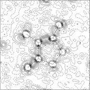
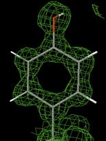
Electron Density Map
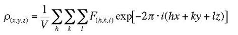
A three-dimensional description of the electron density in a crystal structure, determined from X-ray diffraction experiments. X-rays scatter from the electron clouds of atoms in the crystal lattice; the diffracted waves from scattering planes h,k,l are described by structure factors FhklThe electron density as a function of position x,y,z is the Fourier transform of the structure factors:
![]()
The electron density map describes the contents of the unit cells averaged over the whole crystal and not the contents of a single unit cell (a distinction that is important where structural disorder is present).
Three-dimensional maps are often evaluated as parallel two-dimensional contoured sections at different heights in the unit cell.
Electron density is measured in electrons per cubic ångström, e Å-3.
When X-rays are beamed at the crystal, electrons diffract the X-rays, which causes a diffraction pattern. Using the mathematical Fourier transform these patterns can converted into electron density maps. These maps show contour lines of electron density. Since electrons more or less surround atoms uniformly, it is possible to determine where atoms are located. Unfortunately since hydrogen has only one electron, it is difficult to map hydrogens. To get a three dimensional picture, the crystal is rotated while a computerized detector produces two dimensional electron density maps for each angle of rotation. The third dimension comes from comparing the rotation of the crystal with the series of images. Computer programs use this method to come up with three dimensional spatial coordinates.
Formula (1) implies that the structure factors which we have successfully calculated in the pervious lesson, can be used as Fourier coefficients in an Fourier Summation (or synthesis) to generate the electron density. To be complete, the summation would go from - infinite to + infinite for all indices h,k,l. In reality we have limitations due to the extent to which the diffraction pattern is observed, and the synthesis will be approximate only and may show some truncation effects.
 (1)
(1)
We will caclulate the electron density for our previously calculated structure You need to have the structure saved with a unique file name or the default will be used. In our 1-dimensional case (1) reduces to
which is a real function caclulated from structure factor amplitudes and the corresponding phases. We expect this electron density to show peaks at the atoms positions.
Electron Density Maps
85% of the macromolecular structures available from the Protein Data Bank (PDB) were determined by X-ray crystallography. The direct results of crystallographic experiments are electron density maps. Examining the correspondence between the electron density map and the published molecular model reveals the levels of uncertainty in the model.
An X-ray crystallographic experiment produces an electron density map for the average unit cell of the protein crystal. The amino acid (or nucleotide) sequence of the crystallized polymer(s) is known in advance. The crystallographer fits the atoms of the known molecules into the electron density map, and refines the model and map to the limits of the resolution of the crystal (which is limited by the level of order or disorder in the crystal). The crystallographer then deposits a model of the asymmetric unit of the crystal in the PDB, along with the experimental diffraction data (amplitudes and widths of the X-ray reflection spots, or "structure factors") from which the electron density map can be reconstructed. Electron density maps are available for most PDB files from the Uppsala Electron Density Map Server.
Examining the correspondence between the published model PDB file and the electron density map (EDM) provides much clearer insight into the uncertainties in the model than does merely examining the model itself (see also Quality assessment for molecular models). In addition to examining the entire map (2mFo-DFc) it is revealing to examine the difference map (mFo-DFc), which shows where the model fails to account for the map.
Crystallographers generally use "heavy duty" visualization and modeling software such as Coot or PyMOL, which require considerable practice to use effectively. Jmol first became capable of displaying electron density maps in January, 2010. Being able to display EDM's in Jmol opens the door to examining EDMs effectively in a web browser, with a user interface (yet to be developed) that requires no specialized software knowledge.
The ability to display electron density maps in Proteopedia is under development. Once it becomes possible, interactive maps in Jmol will be shown here. Until then, please see Electron Density Maps in Jmol.
Data submission to PDB
The Worldwide Protein Data Bank (wwPDB) consists of organizations that act as deposition, data processing and distribution centers for PDB data. The founding members are RCSB PDB (USA), PDBe (Europe) and PDBj (Japan). The BMRB (USA) group joined the wwPDB in 2006. The mission of the wwPDB is to maintain a single Protein Data Bank Archive of macromolecular structural data that is freely and publicly available to the global community.
This site provides information about services provided by the individual member organizations and about projects undertaken by the wwPDB. The website address is http://www.wwpdb.org/
The wwPDB will accept all experimentally determined structures of biological macromolecules that meet the minimum requirements. These requirements include: three-dimensional coordinates, information about the composition of the structure (sequence, chemistry, etc.), information about the experiment performed, details of the structure determination steps and author contact information are also necessary for the deposition. In addition, structure factors are required for X-ray submissions and, restraints and chemical shifts are required for NMR submissions.
Since October 15, 2006, PDB depositions are restricted to atomic coordinates that are substantially determined by experimental measurements on actual sample specimens containing biological macromolecules1. Currently, coordinate sets produced by X-ray crystallography, NMR, electron microscopy, neutron diffraction, powder diffraction, fiber diffraction, and solution scattering can be deposited to the PDB, provided the molecule studied meets the minimum size requirement. Theoretical model depositions determined purely in silico using, for example, homology or ab initio methods, are no longer accepted.
Theoretical models that have been previously released or those that were deposited before October 15, 2006 will continue to be publicly available via the historical models archive at ftp://ftp.wwpdb.org/pub/pdb/data/structures/models/.
Data details:
Total data deposited during 2012 is 77758 and processed and released are 69294.
Deposition websites:
he PDB deposition sites for all the experimental methods are available at the following wwPDB sites:
|
RCSB |
http://deposit.rcsb.org/ |
|
PDBe |
http://pdbe.org/deposit/ |
|
PDBj |
http://pdbdep.protein.osaka-u.ac.jp/ |
For NMR model coordinates and experimental data an additional access point is located at:
|
BMRB |
http://deposit.bmrb.wisc.edu/bmrb-adit/ |
|
PDBj-BMRB |
http://nmradit.protein.osaka-u.ac.jp/bmrb-adit/ |
|
PDBe |
http://pdbe.org/deposit/ |
For EM model coordinates and maps data an additional access point is located at:
EMDB http://emdatabank.org/deposit.html
Biomolecular polymers including polypeptides, polynucleotides, polysaccharides, and their complexes that meet the following criteria are accepted:
Crystal structures of peptides with fewer than 24 residues within any polymer chain that do not meet criteria 1, 2, or 3 can be deposited at the Cambridge Crystallographic Data Centre (CCDC, http://www.ccdc.cam.ac.uk/products/csd/deposit/). NMR structures of such molecules can be submitted to Biological Magnetic Resonance Data Bank (BMRB) through the Small Molecule Structure Deposition (SMSdep, http://deposit.bmrb.wisc.edu/bmrb-adit/) system.
Smaller oligonucleotides (dinucleotides and trinucleotides) can be deposited at the Nucleic Acid Database (NDB, http://ndbserver.rutgers.edu).
Molecules that do not conform to these guidelines but have been previously deposited in the PDB will not be removed.
The following data deposition tools and instructions can make your structure deposition easy, complete and accurate:
THEN
The Validation Server can also be used to monitor improvements made to your structural model before you begin the deposition process.
Detailed step-by-step instructions for individual structural methods are available.
The Auto Dep Input Tool (ADIT) was developed by the RCSB for depositing structures to the Protein Data Bank. ADIT also allows the user to check the format of coordinate and structure factor files and to perform a variety of validation tests on a structure prior to deposition in the database. These checks can be done without intervention by the database staff. To deposit a structure, the user uploads the relevant coordinate and structure factor files and then adds any additional information to the submission using ADIT.
To begin a new ADIT session:
Step 1: Data Format Precheck
Step 2: Validation Precheck (Validation)
Step 3: Data Deposition
You may wish to have the following information on hand:
citations of relevant references, sequences of macromolecules in your structure, molecular formulae of ligands, natural or genetic source of macromolecules, crystallization conditions, unit cell, space group, data collection parameters, refinement parameters, rms deviations
Entering information:
Saving the category:
You will be presented with an approximate measure of the completeness of your file for deposition and a table previewing your entry. If you wish to change or add any information, select Return to the Input Tool. If you have added all of the information you would like and do not want to make any changes, press the Deposit Now button. After selecting this button, you will not be able to change the entry any further using ADIT.
A previous ADIT deposition session can be continued at a later date as long as the structure has not been deposited.
To begin a previous ADIT session:
ADIT Validation Server
The ADIT Validation Server allows the user to check the format consistency of coordinates (PRECHECK) and to create validation reports about a structure before deposition (VALIDATION). These checks can be done independently by the user. To start a new validation session, select the experimental method (X-ray or NMR) from the pull-down menu below, and press the BEGIN button.
After submitting your coordinates (and structure factor files, if applicable) you will receive a comprehensive summary report. Examine this RCSB Validation summary letter carefully, since it may indicate outstanding issues that will delay deposition of your coordinates to the PDB.
Website: http://pdb-extract.rcsb.org/auto-check/index-ext.html
SF-Tool Check coordinates against structure factor data and convert various structure factor file formats (formerly Crystallographic Data Validation)
pdb_extract annotation tool Prepare coordinate and structure factor files for deposition Validation server Validate your structure at any time
Protein structure prediction
Protein structure prediction is the prediction of the three-dimensional structure of a protein from its amino acid sequence — that is, the prediction of its secondary, tertiary, and quaternary structure from its primary structure. Structure prediction is fundamentally different from the inverse problem of protein design. Protein structure prediction is one of the most important goals pursued by bioinformatics and theoretical chemistry; it is highly important in medicine (for example, in drug design) and biotechnology (for example, in the design of novel enzymes). Every two years, the performance of current methods is assessed in the CASP experiment (Critical Assessment of Techniques for Protein Structure Prediction).
Secondary structure prediction
Secondary structure prediction is a set of techniques in bioinformatics that aim to predict the local secondary structures of proteins and RNA sequences based only on knowledge of their primary structure — amino acid or nucleotide sequence, respectively. For proteins, a prediction consists of assigning regions of the amino acid sequence as likely alpha helices, beta strands (often noted as "extended" conformations), or turns. The success of a prediction is determined by comparing it to the results of the DSSP algorithm applied to the crystal structure of the protein; for nucleic acids, it may be determined from the hydrogen bonding pattern. Specialized algorithms have been developed for the detection of specific well-defined patterns such as transmembrane helices and coiled coils in proteins, or canonical microRNA structures in RNA.
The best modern methods of secondary structure prediction in proteins reach about 80% accuracy; this high accuracy allows the use of the predictions in fold recognition and ab initio protein structure prediction, classification of structural motifs, and refinement of sequence alignments. The accuracy of current protein secondary structure prediction methods is assessed in weekly benchmarks such as LiveBench and EVA.
The Chou-Fasman method was among the first secondary structure prediction algorithms developed and relies predominantly on probability parameters determined from relative frequencies of each amino acid's appearance in each type of secondary structure. The original Chou-Fasman parameters, determined from the small sample of structures solved in the mid-1970s, produce poor results compared to modern methods, though the parameterization has been updated since it was first published. The Chou-Fasman method is roughly 50-60% accurate in predicting secondary structures.
The GOR method, named for the three scientists who developed it — Garnier, Osguthorpe, and Robson — is an information theory-based method developed not long after Chou-Fasman. It uses a more powerful probabilistic techniques of Bayesian inference. The method is a specific optimized application of mathematics and algorithms developed in a series of papers by Robson and colleagues. The GOR method is capable of continued extension by such principles, and has gone through several versions. The GOR method takes into account not only the probability of each amino acid having a particular secondary structure, but also the conditional probability of the amino acid assuming each structure given the contributions of its neighbors (it does not assume that the neighbors have that same structure). The approach is both more sensitive and more accurate than that of Chou and Fasman because amino acid structural propensities are only strong for a small number of amino acids such as proline and glycine. Weak contributions from each of many neighbors can add up to strong effect overall. The original GOR method was roughly 65% accurate and is dramatically more successful in predicting alpha helices than beta sheets, which it frequently mispredicted as loops or disorganized regions. Later GOR methods considered also pairs of amino acids, significantly improving performance. The major difference from the following technique is perhaps that the weights in an implied network of contributing terms are assigned a priori, from statistical analysis of proteins of known structure, not by feedback to optimize agreement with a training set of such.
Neural network methods use training sets of solved structures to identify common sequence motifs associated with particular arrangements of secondary structures. These methods are over 70% accurate in their predictions, although beta strands are still often underpredicted due to the lack of three-dimensional structural information that would allow assessment of hydrogen bonding patterns that can promote formation of the extended conformation required for the presence of a complete beta sheet.
Support vector machines have proven particularly useful for predicting the locations of turns, which are difficult to identify with statistical methods. The requirement of relatively small training sets has also been cited as an advantage to avoid overfitting to existing structural data.
Extensions of machine learning techniques attempt to predict more fine-grained local properties of proteins, such as backbone dihedral angles in unassigned regions. Both SVMs and neural networks have been applied to this problem.
Secondary structure prediction servers
Secondary Structure prediction
Protein secondary structure prediction refers to the prediction of the conformational state of each amino acid residue of a protein sequence as one of the three possible states, namely, helices, strands, or coils, denoted as H, E, and C, respectively. The prediction is based on the fact that secondary structures have a regular arrangement of amino acids, stabilized by hydrogen bonding patterns. The structural regularity serves the foundation for prediction algorithms.
Because of significant structural differences between globular proteins and transmembrane proteins, they necessitate very different approaches to predicting respective secondary structure elements. Prediction methods for each of two types of proteins are discussed herein. In addition, prediction of supersecondary structures, such as coiled coils, is also described.
Secondary structure for globular protein
Protein secondary structure prediction with high accuracy is not a trivial ask. It remained a very difficult problem for decades. This is because protein secondary structure elements are context dependent. The formation of α-helices is determined by short-range interactions, whereas the formation of β-strands is strongly influenced by long-range interactions. Prediction for long-range interactions is theoretically difficult. After more than three decades of effort, prediction accuracies have only been improved from about 50% to about 75%.
The secondary structure prediction methods can be either ab initio based, which make use of single sequence information only, or homology based, which make use of multiple sequence alignment information. The ab initio methods, which belong to early generation methods, predict secondary structures based on statistical calculations of the residues of a single query sequence. The homology-based methods do not rely on statistics of residues of a single sequence, but on common secondary structural patterns conserved among multiple homologous sequences.
Ab Initio–Based Methods
This type of method predicts the secondary structure based on a single query sequence. It measures the relative propensity of each amino acid belonging to a certain secondary structure element. The propensity scores are derived from known crystal structures. Examples of ab initio prediction are the Chou–Fasman and Garnier, Osguthorpe, Robson (GOR) methods. The ab initio methods were developed in the 1970s when protein structural data were very limited. The statistics derived from the limited data sets can therefore be rather inaccurate. However, the methods are simple enough that they are often used to illustrate the basics of secondary structure prediction.
The Chou–Fasman algorithm (http://fasta.bioch.virginia.edu/fasta/chofas.htm) determines the propensity or intrinsic tendency of each residue to be in the helix, strand, and β-turn conformation using observed frequencies found in protein crystal structures (conformational values for coils are not considered). For example, it is known that alanine, glutamic acid, and methionine are commonly found in α-helices, whereas glycine and proline are much less likely to be found in such structures. The calculation of residue propensity scores is simple. Suppose there are n residues in all known protein structures from which m residues are helical residues. The total number of alanine residues is y of which x are in helices. The propensity for alanine to be in helix is the ratio of the proportion of alanine in helices over the proportion of alanine in over all residue population (using the formula[x/m]/[y/n]). If the propensity for the residue equals 1.0 for helices (P[α-helix]), it means that the residue has an equal chance of being found in helices or elsewhere. If the propensity ratio is less than 1, it indicates that the residue has less chance of being found in helices. If the propensity is larger than 1, the residue is more favored by helices. Based on this concept, Chou and Fasman developed a scoring table listing relative propensities of each amino acid to be in an α-helix, a β-strand, or a β-turn (Table). Prediction with the Chou–Fasman method works by scanning through a sequence with a certain window size to find regions with a stretch of contiguous residues each having a favored SSE score to make a prediction. For α-helices, the window size is six residues, if a region has four contiguous residues each having P(α-helix) > 1.0, it is predicted as an α-helix. The helical region is extended in both directions until the P(α-helix) score becomes smaller than 1.0. That defines the boundaries of the helix. For β-strands, scanning is done with a window size of five residues to search for a stretch of at least three favored β-strand residues. If both types of secondary structure predictions overlap in a certain region, a prediction is made based on the following criterion: if _P(α) > _P(β), it is declared as an α-helix; otherwise, a β-strand. The GOR method (http://fasta.bioch.virginia.edu/fasta www/garnier.htm) is also based on the “propensity” of each residue to be in one of the four conformational states, helix (H), strand(E), turn(T),and coil (C).However, instead of using the propensity value from a single residue to predict a conformational state, it takes short-range interactions of neighboring residues into account. It examines a window of every seventeen residues and sums up propensity scores for all residues for each of the four states resulting in four summed values. The highest scored state defines the conformational state for the center residue in the window (ninth position).The GOR method has been shown to be more accurate than Chou–Fasman because it takes the neighboring effect of residues into consideration. The improvements include more refined residue statistics based on a larger number of solved protein structures and the incorporation of more local residue interactions. Examples of the improved algorithms are GOR II, GOR III, GOR IV, and SOPM. These tools can be found at http://npsa-pbil.ibcp.fr/cgi-bin/npsa automat.pl?page=/NPSA/npsa server.html. These are the second-generation prediction algorithms developed in the 1980s and early 1990s. They have improved accuracy over the first generation by about 10%.
Table: Relative Amino Acid Propensity Values for Secondary Structure Elements Used in the Chou–Fasman Method
Homology-Based Methods
The third generation of algorithms was developed in the late 1990s by making use of evolutionary information. This type of method combines the ab initio secondary structure prediction of individual sequences and alignment information from multiple homologous sequences (>35% identity). The idea behind this approach is that close protein homologs should adopt the same secondary and tertiary structure. When each individual sequence is predicted for secondary structure using a method similar to the GOR method, errors and variations may occur. However, evolutionary conservation dictates that there should be no major variations for their secondary structure elements. Therefore, by aligning multiple sequences, information of positional conservation is revealed. Because residues in the same aligned position are assumed to have the same secondary structure, any inconsistencies or errors in prediction of individual sequences can be corrected using a majority rule (Fig.). This homology based method has helped improve the prediction accuracy by another 10% over the second-generation methods.
Figure : Schematic representation of secondary structure prediction using multiple sequence alignment information. Each individual sequence in the multiple alignment is subject to secondary structure prediction using the GOR method. If variations in predictions occur, they can be corrected by deriving a consensus of the secondary structure elements from the alignment.
Prediction with Neural Networks
The third-generation prediction algorithms also extensively apply sophisticated neural networks (see Chapter 8) to analyze substitution patterns in multiple sequence alignments. As a review, a neural network is a machine learning process that requires a structure of multiple layers of interconnected variables or nodes. Ins econdary structure prediction, the input is an amino acid sequence and the output is the probability of a residue to adopt a particular structure. Between input and output are many connected hidden layers where the machine learning takes place to adjust the mathematical weights of internal connections. The neural network has to be first trained by sequences with known structures so it can recognize the amino acid patterns and their relationships with known structures. During this process, the weight functions in hidden layers are optimized so they can relate input to output correctly. When the sufficiently trained network processes an unknown sequence, it applies the rules learned in training to recognize particular structural patterns.
When multiple sequence alignments and neural networks are combined, the result is further improved accuracy. In this situation, a neural network is trained not by a single sequence but by a sequence profile derived from the multiple sequence alignment. This combined approach has been shown to improve the accuracy to above 75%, which is a breakthrough in secondary structure prediction. The improvement mainly comes from enhanced secondary structure signals through consensus drawing. The following lists several frequently used third generation prediction algorithms available as web servers.
PHD (Profile network from Heidelberg; http://dodo.bioc.columbia.edu/predictprotein/submit def.html) is a web-based program that combines neural network with multiple sequence alignment. It first performs a BLASTP of the query sequence against a nonredundant protein sequence database to find a set of homologous sequences, which are aligned with the MAXHOM program (a weighted dynamic programming algorithm performing global alignment). The resulting alignment in the form of a profile is fed into a neural network that contains three hidden layers. The first hidden layer makes raw prediction based on the multiple sequence alignment by sliding a window of thirteen positions. As in GOR, the prediction is made for the residue in the center of the window. The second layer refines the raw prediction by sliding a window of seventeen positions, which takes into account more flanking positions. This step makes adjustments and corrections of unfeasible predictions from the previous step. The third hidden layer is called the jury network, and contains networks trained in various ways. It makes final filtering by deleting extremely short helices (one or two residues long) and converting them into coils (Fig.). After the correction, the highest scored state defines the conformational state of the residue.
PSIPRED (http://bioinf.cs.ucl.ac.uk/psiform.html) is a web-based program that predicts protein secondary structures using a combination of evolutionary information and neural networks. The multiple sequence alignment is derived from a PSI-BLAST database search. A profile is extracted from the multiple sequence alignment generated from three rounds of automated PSI-BLAST. The profile is then used as input for a neural network prediction similar to that in PHD, but without the jury layer. To achieve higher accuracy, a unique filtering algorithm is implemented to filter out unrelated PSI-BLAST hits during profile construction.
SSpro (http://promoter.ics.uci.edu/BRNN-PRED/) is a web-based program that combines PSI-BLAST profiles with an advanced neural network, known as bidirectional recurrent neural networks (BRNNs). Traditional neural networks are unidirectional, feed-forward systems with the information flowing in one direction from input to output. BRNNs are unique in that the connections of layers are designed to be able to go backward. In this process, known as back propagation, the weights in hidden layers are repeatedly refined. In predicting secondary structure elements, the network uses the sequence profile as input and finds residue correlations by iteratively recycling the network (recursive network). The averaged output from the iterations is given as a final residue prediction. PROTER(http://distill.ucd.ie/porter/) is a recently developed program that uses similar BRNNs and has been shown to slightly out perform SSPRO.
Figure : Schematic representation of secondary structure prediction in the PHD algorithm using neural networks. Multiple sequences derived from the BLAST search are used to compile a profile. The resulting profile is fed into a neural network, which contains three layers – two network layers and one jury layer. The first layer scans thirteen residues per window and makes a raw prediction, which is refined by the second layer, which scans seventeen residues per window. The third layer makes further adjustment to make a final prediction. Adjustment of prediction scores for one amino acid residue is shown.
PROF (Protein forecasting; www.aber.ac.uk/∼phiwww/prof/) is an algorithm that combines PSI-BLAST profiles and a multistaged neural network, similar to that in PHD. In addition, it uses a linear discriminant function to discriminate between the three states.
HMMSTR (Hidden Markov model [HMM] for protein STRuctures; www.bioinfo.rpi.edu/∼bystrc/hmmstr/server.php) uses a branched and cyclic HMM to predict secondary structures. It first breaks down the query sequence into many very short segments (three to nine residues, called I-sites) and builds profiles based on a library of known structure motifs. It then assembles these local motifs into a supersecondary structure. It further uses an HMM with a unique topology linking many smaller HMMs into a highly branched multicyclic form. This is intended to better capture the recurrent local features of secondary structure based on multiple sequence alignment.
Prediction with Multiple Methods
Because no individual methods can always predict secondary structures correctly, it is desirable to combine predictions from multiple programs with the hope of further improving the accuracy. In fact, a number of web servers have been specifically dedicated to making predictions by drawing consensus from results by multiple programs. In many cases, the consensus-based prediction method has been shown to perform slightly better than any single method.
Jpred (www.compbio.dundee.ac.uk/∼www-jpred/) combines the analysis results from six prediction algorithms, including PHD, PREDATOR, DSC, NNSSP, Jnet, and ZPred. The query sequence is first used to search databases with PSI-BLAST for three iterations. Redundant sequence hits are removed. The resulting sequence homologs are used to build a multiple alignment from which a profile is extracted. The profile information is submitted to the six prediction programs. If there is sufficient agreement among the prediction programs, the majority of the prediction is taken as the structure. Where there is no majority agreement in the prediction outputs, the PHD prediction is taken.
PredictProtein (www.embl-heidelberg.de/predictprotein/predictprotein.html) is another multiple prediction server that uses Jpred, PHD, PROF, and PSIPRED, among others. The difference is that the server does not run the individual programs but sends the query to other servers which e-mail the results to the user separately. It does not generate a consensus. It is up to the user to combine multiple prediction results and derive a consensus.
SECONDARY STRUCTURE PREDICTION FOR TRANSMEMBRANE PROTEINS
Transmembrane proteins constitute up to 30%of all cellular proteins. They are responsible for performing a wide variety of important functions in a cell,s uch as signal transduction, cross-membrane transport, and energy conversion. Themembrane proteins are also of tremendous biomedical importance, as they often serve as drug targets for pharmaceutical development.
Prediction of Helical Membrane Proteins
For membrane proteins consisting of transmembrane α–helices, these transmembrane helices are predominantly hydrophobic with a specific distribution of positively charged residues. The α-helices generally run perpendicular to the membrane plane with an average length between seventeen and twenty-five residues. The hydrophobic helices are normally separated by hydrophilic loops with average lengths of fewer than sixty residues. The residues bordering the transmembrane spans are more positively charged. Another feature indicative of the presence of transmembrane segments is that residues at the cytosolic side near the hydrophobic anchor are more positively charged than those at the lumenal or periplasmic side. This is known as the positive-inside rule (Fig. 14.3), which allows the prediction of the orientation of the secondary structure elements. These rules form the basis for transmembrane prediction algorithms.
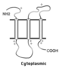
Figure 14.3: Schematic of the positive-inside rule for the orientation of membrane helices. The cylinders represent the transmembrane α–helices. There are relatively more positive charges near the helical anchor on the cytoplasmic side than on the periplasmic side.
A number of algorithms for identifying transmembrane helices have been developed. The early algorithms based their prediction on hydrophobicity scales. They typically scan a window of seventeen to twenty-five residues and assign membrane spans based on hydrophobicity scores. Some are also able to determine the orientation of the membrane helices based on the positive-inside rule. However, predictions solely based on hydrophobicity profiles have high error rates. As with the third-generation predictions for globular proteins, applying evolutionary information with the help of neural networks or HMMs can improve the prediction accuracy significantly. As mentioned, predicting transmembrane helices is relatively easy. The accuracy of someof the best predicting programs, such as TMHMMo r HMMTOP, can exceed 70%. However, the presence of hydrophobic signal peptides can significantly compromise the prediction accuracy because the programs tend to confuse hydrophobic signal peptides with membrane helices. To minimize errors, the presence of signal peptides can be detected using a number of specialized programs and then manually excluded.
TMHMM (www.cbs.dtu.dk/services/TMHMM/) is a web-based program based on an HMM algorithm. It is trained to recognize transmembrane helical patterns based on a training set of 160 well-characterized helical membrane proteins. When a query sequence is scanned, the probability of having an α-helical domain is given. The orientation of the α-helices is predicted based on the positive-inside rule. The prediction output returns the number of transmembrane helices, the boundaries of the helices, and a graphical representation of the helices. This programcan also be used to simply distinguish between globular proteins and membrane proteins.
Phobius (http://phobius.cgb.ki.se/index.html) is a web-based program designed to overcome false positives caused by the presence of signal peptides. The program incorporates distinct HMM models for signal peptides as well as transmembrane helices. After distinguishing the putative signal peptides from the rest of the query sequence, prediction is made on the remainder of the sequence. It has been shown that the prediction accuracy can be significantly improved compared to TMHMM (94% by Phobius compared to 70% by TMHMM). In addition to the normal prediction mode, the user can also define certain sequence regions as signal peptides or other nonmembrane sequences based on external knowledge. As a further step to improve accuracy, the user can perform the “poly prediction” with the PolyPhobius module, which searches the NCBI database for homologs of the query sequence. Prediction for the multiple homologous sequences helps to derive a consensus prediction. However, this option is also more time consuming.
Prediction of β-Barrel Membrane Proteins
For membrane proteins with β-strands only, the β-strands forming the transmembrane segment are amphipathic in nature. They contain ten to twenty-two residues with every second residue being hydrophobic and facing the lipid bilayers whereas the other residues facing the pore of the β-barrel are more hydrophilic. Obviously, scanning a sequence by hydrophobicity does not reveal transmembrane β-strands. These programs for predicting transmembrane α-helices are not applicable for this unique type of membrane proteins. To predict the β-barrel type of membrane proteins, a small number of algorithms have been made available based on neural networks and related techniques.
TBBpred (www.imtech.res.in/raghava/tbbpred/) is a web server for predicting transmembrane β-barrel proteins. It uses a neural network approach to predict transmembrane β-barrel regions. The network is trained with the known structural information of a limited number of transmembrane β-barrel protein structures. The algorithm contains a single hidden layer with five nodes and a single output node. In addition to neural networks, the server can also predict using a support vector machine (SVM) approach, another type of statistical learning process. Similar to neural networks, in SVM the data are fed into kernels (similar to nodes), which are separated into different classes by a “hyperplane” (an abstract linear or nonlinear separator) according to a particular mathematical function. It has the advantage over neural networks in that it is faster to train and more resistant to noise.
COILED COIL PREDICTION
Coiled coils are superhelical structures involving two to more interacting α-helices from the same or different proteins. The individual α-helices twist and wind around each other to form a coiled bundle structure. The coiled coil conformation is important in facilitating inter- or intraprotein interactions. Proteins possessing these structural domains are often involved in transcription regulation or in the maintenance of cytoskeletal integrity.
Coiled coils have an integral repeat of seven residues (heptads) which assume a side-chain packing geometry at facing residues. For every seven residues, the first and fourth are hydrophobic, facing the helical interface; the others are hydrophilic and exposed to the solvent (Fig.). The sequence periodicity forms the basis for designing algorithms to predict this important structural domain. As a result of the regular structural features, if the location of coiled coils can be predicted precisely, the three-dimensional structure for the coiled coil region can sometimes be built. The following lists several widely used programs for the specialized prediction.
Coils (www.ch.embnet.org/software/COILS form.html) is a web-based program that detects coiled coil regions in proteins. It scans a window of fourteen, twentyone, or twenty-eight residues and compares the sequence to a probability matrix compiled from known parallel two-stranded coiled coils. By comparing the similarity scores, the program calculates the probability of the sequence to adopt a coiled coil conformation. The program is accurate for solvent-exposed, left-handed coiled coils, but less sensitive for other types of coiled coil structures, such as buried or righthanded coiled coils.
Multicoil (http://jura.wi.mit.edu/cgi-bin/multicoil/multicoil.pl) is a web-based program for predicting coiled coils. The scoring matrix is constructed based on a database of known two-stranded and three-stranded coiled coils. The program is more conservative than Coils. It has been recently used in several genome-wide studies to screen for protein–protein interactions mediated by coiled coil domains. Leucine zipper domains are a special type of coiled coils found in transcription regulatory proteins. They contain two antiparallel α-helices held together by hydrophobic interactions of leucine residues. The heptad repeat pattern is L-X(6)-L-X(6)-L–X(6)-L. This repeat pattern alone can sometimes allow the domain detection, albeit with high rates of false positives. The reason for the high false-positive rates is that the condition of the sequence region being a coiled coil conformation is not satisfied. To address this problem, algorithms have been developed that take into account both leucine repeats and coiled coil conformation to give accurate prediction.
2ZIP (http://2zip.molgen.mpg.de/) is aweb-based server that predicts leucine zippers. It combines searching of the characteristic leucine repeats with coiled coil prediction using an algorithm similar to Coils to yield accurate results.
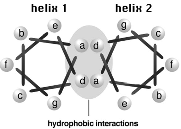
Figure: Cross-section view of a coiled coil structure. A coiled coil protein consisting of two interacting helical strands is viewed from top. The bars represent covalent bonds between amino acid residues. There is no covalent bond between residue a and g. The bar connecting the two actually means to connect the first residue of the next heptad. The coiled coil has a repeated seven residue motif in the form of a-b-c-d-e-f-g. The first and fourth positions (a and d) are hydrophobic, whose interactions with corresponding residues in another helix stabilize the structure. The positions b, c, e, f, g are hydrophilic and are exposed on the surface of the protein.
Tertiary structure prediction
The practical role of protein structure prediction is now more important than ever. Massive amounts of protein sequence data are produced by modern large-scale DNA sequencing efforts such as the Human Genome Project. Despite community-wide efforts in structural genomics, the output of experimentally determined protein structures—typically by time-consuming and relatively expensive X-ray crystallography or NMR spectroscopy—is lagging far behind the output of protein sequences. The protein structure prediction remains an extremely difficult and unresolved undertaking. The two main problems are calculation of protein free energy and finding the global minimum of this energy. A protein structure prediction method must explore the space of possible protein structures which is astronomically large. These problems can be partially bypassed in "comparative" or homology modeling and fold recognition methods, when the search space is pruned by the assumption that the protein in question adopts a structure that is close to the experimentally determined structure of another homologous protein. On the other hand, the de novo or ab initio protein structure prediction methods must explicitly resolve these problems.
Ab initio- or de novo- protein modelling methods seek to build three-dimensional protein models "from scratch", i.e., based on physical principles rather than (directly) on previously solved structures. There are many possible procedures that either attempt to mimic protein folding or apply some stochastic method to search possible solutions (i.e., global optimization of a suitable energy function). These procedures tend to require vast computational resources, and have thus only been carried out for tiny proteins. To predict protein structure de novo for larger proteins will require better algorithms and larger computational resources like those afforded by either powerful supercomputers (such as Blue Gene or MDGRAPE-3) or distributed computing (such as Folding@home, the Human Proteome Folding Project and Rosetta@Home). Although these computational barriers are vast, the potential benefits of structural genomics (by predicted or experimental methods) make ab initio structure prediction an active research field.
Comparative protein modelling
Comparative protein modelling uses previously solved structures as starting points, or templates. This is effective because it appears that although the number of actual proteins is vast, there is a limited set of tertiary structural motifs to which most proteins belong. It has been suggested that there are only around 2,000 distinct protein folds in nature, though there are many millions of different proteins.
These methods may also be split into two groups
Homology modeling is based on the reasonable assumption that two homologous proteins will share very similar structures. Because a protein's fold is more evolutionarily conserved than its amino acid sequence, a target sequence can be modeled with reasonable accuracy on a very distantly related template, provided that the relationship between target and template can be discerned through sequence alignment. It has been suggested that the primary bottleneck in comparative modelling arises from difficulties in alignment rather than from errors in structure prediction given a known-good alignment. Unsurprisingly, homology modelling is most accurate when the target and template have similar sequences.
Protein threading scans the amino acid sequence of an unknown structure against a database of solved structures. In each case, a scoring function is used to assess the compatibility of the sequence to the structure, thus yielding possible three-dimensional models. This type of method is also known as 3D-1D fold recognition due to its compatibility analysis between three-dimensional structures and linear protein sequences. This method has also given rise to methods performing an inverse folding search by evaluating the compatibility of a given structure with a large database of sequences, thus predicting which sequences have the potential to produce a given fold.
Tertiary structure prediction servers:
Homology modeling
Threading
Ab initio
Tertiary structure prediction
There are three computational approaches to protein three-dimensional structural modeling and prediction. They are homology modeling, threading, and ab initio prediction. The first two are knowledge-based methods; they predict protein structures based on knowledge of existing protein structural information in databases. Homology modeling builds an atomic model based on an experimentally determined structure that is closely related at the sequence level. Threading identifies proteins that are structurally similar, with or without detectable sequence similarities. The ab initio approach is simulation based and predicts structures based on physicochemical principles governing protein folding without the use of structural templates.
Homology modeling
As the name suggests, homology modeling predicts protein structures based on sequence homology with known structures. It is also known as comparative modeling. The principle behind it is that if two proteins share a high enough sequence similarity, they are likely to have very similar three-dimensional structures. If one of the protein sequences has a known structure, then the structure can be copied to the unknown protein with a high degree of confidence. Homology modeling produces an all-atom model based on alignment with template proteins. The overall homology modeling procedure consists of six steps. The first step is template selection, which involves identification of homologous sequences in the protein structure database to be used as templates for modeling. The second step is alignment of the target and template sequences. The third step is to build a framework structure for the target protein consisting of main chain atoms. The fourth step of model building includes the addition and optimization of side chain atoms and loops. The fifth step is to refine and optimize the entire model according to energy criteria. The final step involves evaluating of the overall quality of the model obtained (Fig.). If necessary, alignment and model building are repeated until a satisfactory result is obtained.
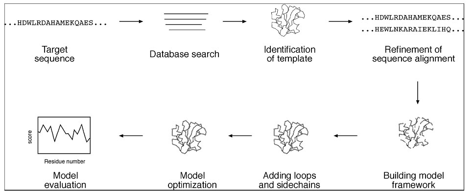
Flowchart showing steps involved in homology modeling.
Template Selection
The first step in protein structural modeling is to select appropriate structural templates. This forms the foundation for rest of the modeling process. The template selection involves searching the Protein Data Bank (PDB) for homologous proteins with determined structures. The search can be performed using a heuristic pairwise alignment search program such as BLAST or FASTA. However, the use of dynamic programming based search programs such as SSEARCH or ScanPS can result in more sensitive search results. The relatively small size of the structural database means that the search time using the exhaustive method is still within reasonable limits, while giving a more sensitive result to ensure the best possible similarity hits.
Sequence Alignment
Once the structure with the highest sequence similarity is identified as a template, the full-length sequences of the template and target proteins need to be realigned using refined alignment algorithms to obtain optimal alignment. This realignment is the most critical step in homology modeling, which directly affects the quality of the final model. This is because incorrect alignment at this stage leads to incorrect designation of homologous residues and therefore to incorrect structural models. Errors made in the alignment step cannot be corrected in the following modeling steps. Therefore, the best possible multiple alignment algorithms, such as Praline and T-Coffee, should be used for this purpose.
Backbone Model Building
Once optimal alignment is achieved, residues in the aligned regions of the target protein can assume a similar structure as the template proteins, meaning that the coordinates of the corresponding residues of the template proteins can be simply copied onto the target protein. If the two aligned residues are identical, coordinates of the side chain atoms are copied along with the main chain atoms. If the two residues differ, only the backbone atoms can be copied. The side chain atoms are rebuilt in a subsequent procedure.
Loop Modeling
In the sequence alignment for modeling, there are often regions caused by insertions and deletions producing gaps in sequence alignment. The gaps cannot be directly modeled, creating “holes” in the model. Closing the gaps requires loop modeling, which is a very difficult problem in homology modeling and is also a major source of error. Loop modeling can be considered a mini–protein modeling problem by itself. Unfortunately, there are no mature methods available that can model loops reliably. Currently, there are two main techniques used to approach the problem: the database searching method and the ab initio method.
The database method involves finding “spare parts” from known protein structures in a database that fit onto the two stem regions of the target protein. The stems are defined as the main chain atoms that precede and follow the loop to be modeled. The procedure begins by measuring the orientation and distance of the anchor regions in the stems and searching PDB for segments of the same length that also match the above endpoint conformation. Usually, many different alternative segments that fit the endpoints of the stems are available. The best loop can be selected based on sequence similarity as well as minimal steric clashes with the neighboring parts of the structure. The conformation of the best matching fragments is then copied onto the anchoring points of the stems. The ab initio method generates many random loops and searches for the one that does not clash with nearby side chains and also has reasonably low energy and φ and ψ angles in the allowable regions in the Ramachandran plot.
If the loops are relatively short (three to five residues), reasonably correct models can be built using either of the two methods. If the loops are longer, it is very difficult to achieve a reliable model. The following are specialized programs for loop modeling.
FREAD (www-cryst.bioc.cam.ac.uk/cgi-bin/coda/fread.cgi) is a web server that models loops using the database approach.
PETRA (www-cryst.bioc.cam.ac.uk/cgi-bin/coda/pet.cgi) is aweb server that uses the ab initio method to model loops.
CODA (www-cryst.bioc.cam.ac.uk/∼charlotte/Coda/search coda.html) is a web server that uses a consensus method based on the prediction results from FREAD and PETRA. For loops of three to eight residues, it uses consensus conformation of both methods and for nine to thirty residues, it uses FREAD prediction only.
Side Chain Refinement
Once main chain atoms are built, the positions of side chains that are not modeled must be determined. Modeling side chain geometry is very important in evaluating protein–ligand interactions at active sites and protein–protein interactions at the contact interface. A side chain can be built by searching every possible conformation at every torsion angle of the side chain to select the one that has the lowest interaction energy with neighboring atoms. However, this approach is computationally prohibitive in most cases. In fact, most current side chain prediction programs use the concept of rotamers, which are favored side chain torsion angles extracted from known protein crystal structures. A collection of preferred side chain conformations is a rotamer library in which the rotamers are ranked by their frequency of occurrence. Having a rotamer library reduces the computational time significantly because only a small number of favored torsion angles are examined. In prediction of side chain conformation, only the possible rotamers with the lowest interaction energy with nearby atoms are selected.
Most modeling packages incorporate the side chain refinement function. A specialized side chain modeling program that has reasonably good performance is SCWRL (sidechain placement with a rotamer library; www.fccc.edu/research/labs/ dunbrack/scwrl/), a UNIX program that works by placing side chains on a backbone template according to preferences in the backbone-dependent rotamer library. It removes rotamers that have steric clashes with main chain atoms. The final, selected set of rotamers has minimal clashes with main chain atoms and other side chains.
Model Refinement Using Energy Function
In these loop modeling and side chain modeling steps, potential energy calculations are applied to improve the model. However, this does not guarantee that the entire raw homology model is free of structural irregularities such as unfavorable bond angles, bond lengths, or close atomic contacts. These kinds of structural irregularities can be corrected by applying the energy minimization procedure on the entire model, which moves the atoms in such a way that the overall conformation has the lowest energy potential. The goal of energy minimization is to relieve steric collisions and strains without significantly altering the overall structure.
However, energy minimization has to be used with caution because excessive energy minimization often moves residues away from their correct positions. Therefore, only limited energy minimization is recommended (a few hundred iterations) to remove major errors, such as short bond distances and close atomic clashes. Key conserved residues and those involved in cofactor binding have to be restrained if necessary during the process.
Another often used structure refinement procedure is molecular dynamic simulation. This practice is derived from the concern that energy minimization only moves atoms toward a local minimum without searching for all possible conformations, often resulting in a suboptimal structure. To search for a global minimum requires moving atoms uphill as well as downhill in a rough energy landscape. This requires thermodynamic calculations of the atoms. In this process, a protein molecule is “heated” or “cooled” to simulate the uphill and downhill molecular motions. Thus, it helps overcome energy hurdles that are inaccessible to energy minimization. It is hoped that this simulation follows the protein folding process and has a better chance at finding the true structure. A more realistic simulation can include water molecules surrounding the structure. This makes the process an even more computationally expensive procedure than energy minimization, however. Furthermore, it shares a similar weakness of energy minimization: a molecular structure can be “loosened up” such that it becomes less realistic. Much caution is therefore needed in using these molecular dynamic tools.
GROMOS (www.igc.ethz.ch/gromos/) is a UNIX program for molecular dynamic simulation. It is capable of performing energy minimization and thermodynamic
Model Evaluation
The final homology model has to be evaluated to make sure that the structural features of the model are consistent with the physicochemical rules. This involves checking anomalies in φ–ψ angles, bond lengths, close contacts, and so on. Another way of checking the quality of a protein model is to implicitly take these stereochemical properties into account. This is a method that detects errors by compiling statistical profiles of spatial features and interaction energy from experimentally determined structures. By comparing the statistical parameters with the constructed model, the method reveals which regions of a sequence appear to be folded normally and which regions do not. If structural irregularities are found, the region is considered to have errors and has to be further refined.
Procheck (www.biochem.ucl.ac.uk/∼roman/procheck/procheck.html) is a UNIX program that is able to check general physicochemical parameters such as φ–ψ angles, chirality, bond lengths, bond angles, and so on. The parameters of the model are used to compare with those compiled from well-defined, high-resolution structures.
If the program detects unusual features, it highlights the regions that should be checked or refined further.
WHAT IF (www.cmbi.kun.nl:1100/WIWWWI/) is a comprehensive protein analysis server that validates a protein model for chemical correctness. It has many functions, including checking of planarity, collisions with symmetry axes (close contacts), proline puckering, anomalous bond angles, and bond lengths. It also allows the generation of Ramachandran plots as an assessment of the quality of the model.
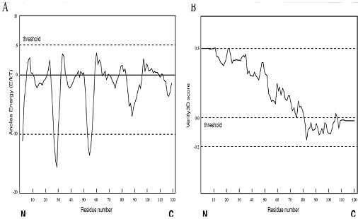
Figure: Example of protein model evaluation outputs by ANOLEA and Verify3D. The protein model was obtained from the Swiss model database (model code 1n5d). (A) The assessment result by the ANOLEA server. The threshold for unfavorable residues is normally set at 5.0. Residues with scores above 5.0 are considered regions with errors. (B) The assessment result by the Verify3D server. The threshold value is normally set at zero. The residues with the scores below zero are considered to have an unfavorable environment.
ANOLEA (Atomic Non-Local Environment Assessment; http://protein.bio.puc.cl/cardex/servers/anolea/index.html) is a web server that uses the statistical evaluation approach. It performs energy calculations for atomic interactions in a protein chain and compares these interaction energy values with those compiled from a database of protein x-ray structures. If the energy terms of certain regions deviate significantly from those of the standard crystal structures, it defines them as unfavorable regions. An example of the output from the verification of a homology model. The threshold for unfavorable residues is normally set at 5.0. Residues with scores above 5.0 are considered regions with errors.
Verify3D (www.doe-mbi.ucla.edu/Services/Verify 3D/) is another server using the statistical approach. It uses a precomputed database containing eighteen environmental profiles based on secondary structures and solvent exposure, compiled from high-resolution protein structures. To assess the quality of a protein model, the secondary structure and solvent exposure propensity of each residue are calculated. If the parameters of a residue fall within one of the profiles, it receives a high score, otherwise a low score. The result is a two-dimensional graph illustrating the folding quality of each residue of the protein structure. A verification output of the above homology model is shown in Figure. The threshold value is normally set at zero. Residues with scores below zero are considered to have an unfavorable environment. The assessment results can be different using different verification programs. As showninFigure, ANOLEA appears to be less stringent thanVerify3D. Although the full-length protein chain of this model is declared favorable by ANOLEA, residues in the C-terminus of the protein are considered to be of lowquality by Verify3D. Because no single method is clearly superior to any other, a good strategy is to use multiple verification methods and identify the consensus between them. It is also important to keep in mind that the evaluation tests performed by these programs only check the stereochemical correctness, regardless of the accuracy of the model, which may or may not have any biological meaning.
ERRAT. The ERRAT program has already been described. It analyzes on bonded atom contacts in protein structures in terms of CC, CN, CO, and so forth contacts.
QUALITY INFORMATION ON THE WEB
Rather than having to install and run one of the above packages, it is possible to obtain much of the information they provide from the Web. Several sites provide precomputed quality criteria for all existing structures in the PDB. Other sites allow you upload your own PDB file, via your Web browser, and will run their validation programs on it and provide you with the results of their checks.
PDBsum—PROCHECK Summaries
The first site that provides precomputed quality criteria is the PDBsum Web site at http://www.biochem.ucl.ac.uk/bsm/pdbsum. This Web site specializes in structural analyses and pictorial representations of all PDB structures. Each structure containing one or more protein chains has a PROCHECK and a WHATCHECK button. The former gives a Ramachandran plot for all protein chains in the structure, together with summary statistics calculated by the PROCHECK program.
These results can provide a quick guide to the likely quality of the structure, in addition to the structure’s resolution, R-factor and, where available, Rfree.
The WHATCHECK button links to the PDBREPORT for the structure, described below. Occasionally the model of a protein structure is so bad that one can tell immediately from merely looking at the secondary structure plot on the PDBsum page. Most proteins have around 50–60% of their residues in regions of regular secondary structure, that is, in α-helices and β –strands. However, if a model is really poor, the main-chain oxygen and nitrogen atoms responsible for the hydrogen-bonding that maintains the regular secondary structures can lie beyond normal hydrogen-bonding distances; so the algorithms that assign secondary structure may fail to detect some of the α-helices and β –strands that the correct protein structure contains.
PDBREPORT—WHATCHECK Results
The WHATCHECK button on the PDBsum page leads to the WHAT IF Check report on the given protein’s coordinates. This report is a detailed listing (plus an even more detailed one, called the Full report) of the numerous analyses that have been precomputed using the WHATCHECK program. These analyses include space group and symmetry checks, geometrical checks on bond lengths, bond angles, torsion angles, proline puckers, bad contacts, planarity checks, checks on hydrogen-bonds, and more, including an overall summary report intended for users of the model. The PDBREPORT database can be accessed directly at http://www.cmbi.kun.nl/gv/pdbreport.
PDB’s Geometry Analyses
The PDB Web site (http://www.rcsb.org/pdb) also has geometrical analyses on each entry, consisting of tables of average, minimum, and maximum values for the protein’s bond lengths, bond angles, and dihedral angles. Unusual values are highlighted. It is also possible to view a backbone representation of the structure in RasMol, colored according to the Fold Deviation Score—the redder the coloring the more unusual the residue’s conformational parameters.
Comprehensive Modeling Programs
A number of comprehensive modeling programs are able to perform the complete procedure of homology modeling in an automated fashion. The automation requires assembling a pipeline that includes target selection, alignment, model generation, and model evaluation. Some freely available protein modeling programs and servers are listed.
Modeller (http://bioserv.cbs.cnrs.fr/HTML BIO/frame mod.html) is a web server for homology modeling. The user provides a predetermined sequence alignment of a template(s) and a target to allow the program to calculate a model containing all of the heavy atoms (nonhydrogen atoms). The program models the backbone using a homology-derived restraint method, which relies on multiple sequence alignment between target and template proteins to distinguish highly conserved residues from less conserved ones. Conserved residues are given high restraints in copying from the template structures. Less conserved residues, including loop residues, are given less or no restraints, so that their conformations can be built in a more or less ab initio fashion. The entire model is optimized by energy minimization and molecular dynamics procedures.
Swiss-Model (www.expasy.ch/swissmod/SWISS-MODEL.html) is an automated modeling server that allows a user to submit a sequence and to get back a structure automatically. The server constructs a model by automatic alignment (First Approach mode) or manual alignment (Optimize mode). In the First Approach mode, the user provides sequence input for modeling. The server performs alignment of the query with sequences in PDB using BLAST. After selection of suitable templates, a raw model is built. Refinement of the structure is done using GROMOS. Alternatively, the user can specify or upload structures as templates. The final model is sent to the user by e-mail. In the Optimize mode, the user constructs a sequence alignment in SwissPdbViewer and submits it to the server for model construction.
3D-JIGSAW (www.bmm.icnet.uk/servers/3djigsaw/) is a modeling server that works in either the automatic mode or the interactive mode. Its loop modeling relies on the database method. The interactive mode allows the user to edit alignments and select templates, loops, and side chains during modeling, whereas the automatic mode allows no human intervention and models a submitted protein sequence if it has an identity >40% with known protein structures.
THREADING AND FOLD RECOGNITION
There are only small number of protein folds available (<1,000), compared to millions of protein sequences. This means that protein structures tend to be more conserved than protein sequences. Consequently, many proteins can share a similar fold even in the absence of sequence similarities. This allowed the development of computational methods to predict protein structures beyond sequence similarities. To determine whether a protein sequence adopts a known three-dimensional structure fold relies on threading and fold recognition methods.
By definition, threading or structural fold recognition predicts the structural fold of an unknown protein sequence by fitting the sequence into a structural database and selecting the best-fitting fold. The comparison emphasizes matching of secondary structures, which are most evolutionarily conserved. Therefore, this approach can identify structurally similar proteins even without detectable sequence similarity. The algorithms can be classified into two categories, pairwise energy based and profile based. The pairwise energy–based method was originally referred to as threading and the profile-based method was originally defined as fold recognition. However, the two terms are now often used interchangeably without distinction in the literature.
Pairwise Energy Method
In the pairwise energy based method, aprotein sequence is searched for in a structural fold database to find the best matching structural fold using energy-based criteria. The detailed procedure involves aligning the query sequence with each structural fold in a fold library. The alignment is performed essentially at the sequence profile level using dynamic programming or heuristic approaches. Local alignment is often adjusted to get lower energy and thus better fitting. The adjustment can be achieved using algorithms such as double-dynamic programming. The next step is to build a crude model for the target sequence by replacing aligned residues in the template structure with the corresponding residues in the query. The third step is to calculate the energy terms of the raw model, which include pairwise residue interaction energy, solvation energy, and hydrophobic energy. Finally, the models are ranked based on the energy terms to find the lowest energy fold that corresponds to the structurally most compatible fold (Fig.).
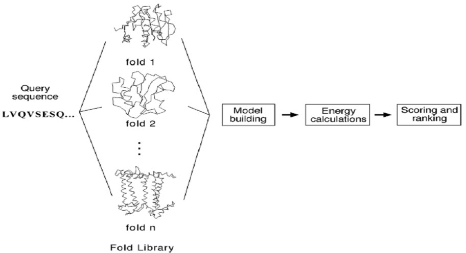
Figure: Outline of the threading method using the pairwise energy approach to predict protein structural folds from sequence. By fitting a structural fold library and assessing the energy terms of the resulting raw models, the best-fit structural fold can be selected.
Profile Method
In the profile-based method, a profile is constructed for a group of related protein structures. The structural profile is generated by superimposition of the structures to expose corresponding residues. Statistical information from these aligned residues is then used to construct a profile. The profile contains scores that describe the propensity of each of the twenty amino acid residues to be at each profile position. The profile scores contain information for secondary structural types, the degree of solvent exposure, polarity, and hydrophobicity of the amino acids. To predict the structural fold of an unknown query sequence, the query sequence is first predicted for its secondary structure, solvent accessibility, and polarity. The predicted information is then used for comparison with propensity profiles of known structural folds to find the fold that best represents the predicted profile.
Because threading and fold recognition detect structural homologs without completely relying on sequence similarities, they have been shown to be far more sensitive than PSI-BLAST in finding distant evolutionary relationships. In many cases, they can identify more than twice as many distant homologs than PSI-BLAST. However, this high sensitivity can also be their weakness because high sensitivity is often associated with low specificity. The predictions resulting from threading and fold recognition often come with very high rates of false positives. Therefore, much caution is required in accepting the prediction results. Threading and fold recognition assess the compatibility of an amino acid sequence with a known structure ina fold library. If the protein fold to be predicted does not exist in the fold library, the method will fail. Another disadvantage compared to homology modeling lies in the fact that threading and fold recognition do not generate fully refined atomic models for the query sequences. This is because accurate alignment between distant homologs is difficult to achieve. Instead, threading and fold recognition procedures only provide a rough approximation of the overall topology of the native structure.
A number of threading and fold recognition programs are available using either or both prediction strategies. At present, no single algorithm is always able to provide reliable fold predictions. Some algorithms work well with some types of structures, but fail with others. It is a good practice to compare results from multiple programs for consistency and judge the correctness by using external knowledge.
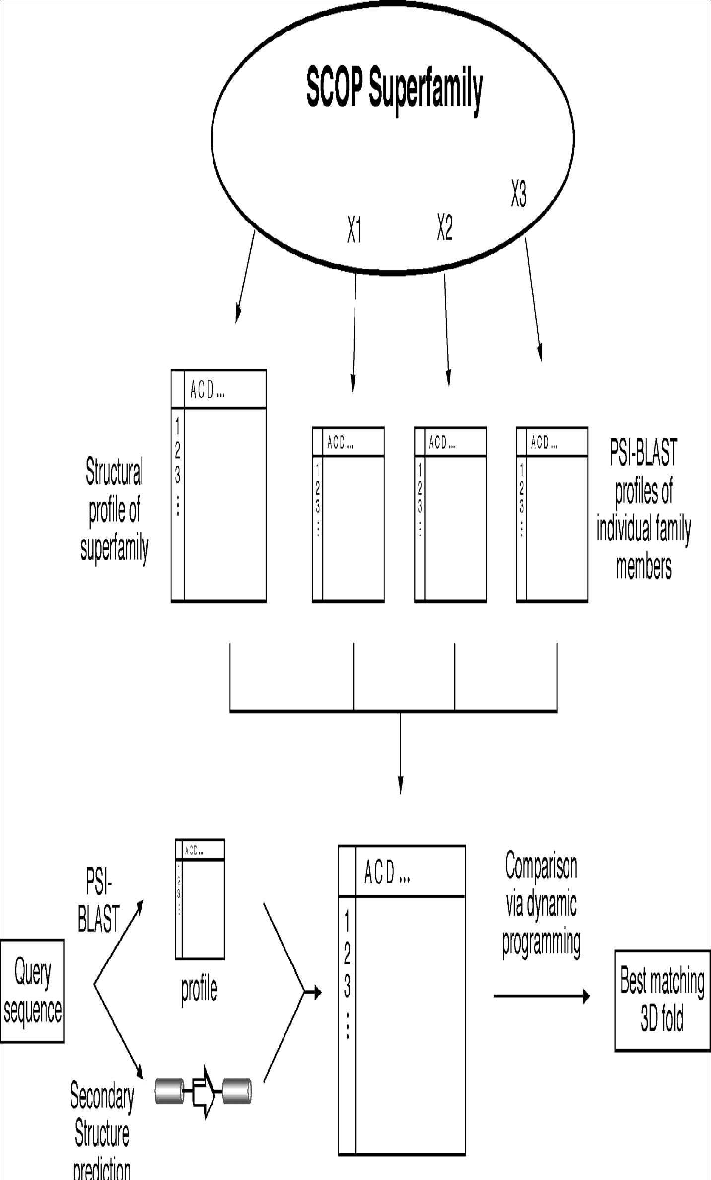
Figure: Schematic diagram of fold recognition by 3D-PSSM. A profile for protein structures in a SCOP superfamily is precomputed based on the structure profile of all members of the superfamily, as well as on PSI-BLAST sequence profiles of individual members of the superfamily. For the query sequence, a PSI-BLAST profile is constructed and its secondary structure information is predicted, which together are used to compare with the precomputed protein superfamily profile.
3D-PSSM (www.bmm.icnet.uk/∼3dpssm/) is a web-based program that employs the structural profile method to identify protein folds. The profiles for each protein superfamily are constructed by combining multiple smaller profiles. First, protein structures in a superfamily based on the SCOP classification are superimposed and are used to construct a structural profile by incorporating secondary structures and solvent accessibility information for corresponding residues. In addition, each member in a protein structural superfamily has its own sequence-based PSI-BLAST profile computed. These sequence profiles are used in combination with the structure profile to forma large superfamily profile in which each position contains both sequence and structural information. For the query sequence, PSI-BLAST is performed to generate a sequence-based profile. PSI-PRED is used to predict its secondary structure. Both the sequence profile and predicted secondary structure are compared with the precomputed protein superfamily profiles, using a dynamic programming approach. The matching scores are calculated in terms of secondary structure, salvation energy, and sequence profiles and ranked to find the highest scored structure fold (Fig.).
GenThreader (http://bioinf.cs.ucl.ac.uk/psipred/index.html) is a web-based program that uses a hybrid of the profile and pairwise energy methods. The initial step is similar to 3D-PSSM; the query protein sequence is subject to three rounds of PSI-BLAST. The resulting multiple sequence hits are used to generate a profile. Its secondary structure is predicted using PSIPRED. Both are used as input for threading computation based on a pairwise energy potential method. The threading results are evaluated using neural networks that combine energy potentials, sequence alignment scores, and length information to create a single score representing the relationship between the query and template proteins.
Fugue (www-cryst.bioc.cam.ac.uk/∼fugue/prfsearch.html) is a profile-based fold recognition server. It has precomputed structural profiles compiled from multiple alignments of homologous structures, which take into account local structural environment such as secondary structure, solvent accessibility, and hydrogen bonding status. The query sequence (or a multiple sequence alignment if the user prefers) is used to scan the database of structural profiles. The comparison between the query and the structural profiles is done using global alignment or local alignment depending on sequence variability.
AB INITIO PROTEIN STRUCTURAL PREDICTION
Both homology and fold recognition approaches rely on the availability of template structures in the database to achieve predictions. If no correct structures exist in the database, the methods fail. However, proteins in nature fold on their own without checking what the structures of their homologs are in databases. Obviously, there is some information in the sequences that provides instruction for the proteins to “find” their native structures. Early biophysical studies have shown that most proteins fold spontaneously into a stable structure that has near minimum energy. This structural state is called the native state. This folding process appears tobenonrandom;however, its mechanism is poorly understood.
The limited knowledge of protein folding forms the basis of ab initio prediction. As the name suggests, the ab initio prediction method attempts to produce all-atom protein models based on sequence information alone without the aid of known protein structures. The perceived advantage of this method is that predictions are not restricted by known folds and that novel protein folds can be identified. However, because the physicochemical laws governing protein folding are not yet well understood, the energy functions used in the ab initio prediction are at present rather inaccurate. The folding problem remains one of the greatest challenges in bioinformatics today.
Current ab initio algorithms are not yet able to accurately simulate the protein folding process. They work by using some type of heuristics. Because the native state of a protein structure is near energy minimum, the prediction programs are thus designed using the energy minimization principle. These algorithms search for every possible conformation to find the one with the lowest global energy. However, searching for a fold with the absolute minimum energy may not be valid in reality. This contributes to one of the fundamental flaws of this approach. In addition, searching for all possible structural conformations is not yet computationally feasible. It has been estimated that, by using one of the world’s fastest supercomputers (one trillion operations per second), it takes 10 20 years to sample all possible conformations of a 40-residue protein. Therefore, some type of heuristics must be used to reduce the conformational space to be searched. Some recent ab initio methods combine fragment search and threading to yield a model of an unknown protein. The following web program is such an example using the hybrid approach.
Rosetta (www.bioinfo.rpi.edu/∼bystrc/hmmstr/server.php) is a web server that predicts protein three-dimensional conformations using the ab initio method. This in fact relies on a “mini-threading” method. The method first breaks down the query sequence into many very short segments (three to nine residues) and predict the secondary structure of the small segments using a hiddenMarkov model–based program, HMMSTR. The segments with assigned secondary structures are subsequently assembled into a three-dimensional configuration. Through random combinations of the fragments, a large number of models are built and their overall energy potentials calculated. The conformation with the lowest global free energy is chosen as the best model.
It needs to be emphasized that up to now, ab initio prediction algorithms are far from mature. Their prediction accuracies are too low to be considered practically useful. Ab initio prediction of protein structures remains a fanciful goal for the future. However, with the current pace of high-throughput structural determination by the structural proteomics initiative, which aims to solve all protein folds within a decade, the time may soon come when there is little need to use the ab initio modeling approach because homology modeling and threading can provide much higher quality predictions for all possible protein folds. Regardless of the progress made in structural proteomics, exploration of protein structures using the ab initio prediction approach may still yield insight into the protein-folding process.
CASP
Discussion of protein structural prediction would not be complete without mentioning CASP (Critical Assessment of Techniques for Protein Structure Prediction). With so many protein structure prediction programs available, there is a need to know the reliability of the prediction methods. For that purpose, a common benchmark is needed to measure the accuracies of the prediction methods. To avoid letting programmers know the correct answer in the structure benchmarks in advance, already published protein structures cannot be used for testing the efficacy of new methodologies. Thus, a biannual international contest was initiated in 1994. It allows developers to predict unknown protein structures through blind testing so that the reliability of new prediction methods can be objectively evaluated. This is the experiment of CASP.
CASP contestants are given protein sequences whose structures have been solved by x-ray crystallography and NMR, but not yet published. Each contestant predicts the structures and submits the results to the CASP organizers before the structures are made publicly available. The results of the predictions are compared with the newly determined structures using structure alignment programs such as VAST, SARF, and DALI. In this way, new prediction methodologies can be evaluated without the possibility of bias. The predictions can be made at various levels of detail (secondary or tertiary structures) and in various categories (homology modeling, threading, ab initio). This experiment has been shown to provide valuable insight into the performance of prediction methods and has become the major driving force of development for protein structure prediction methods. For more information, the reader is recommended to visit the web site of the Protein Structure Prediction Center at http://predictioncenter.llnl.gov/.
Molecular Modeling (Molecular Design)
Molecular modelling encompasses all theoretical methods and computational techniques used to model or mimic the behaviour of molecules. The techniques are used in the fields of computational chemistry, computational biology and materials science for studying molecular systems ranging from small chemical systems to large biological molecules and material assemblies. The simplest calculations can be performed by hand, but inevitably computers are required to perform molecular modelling of any reasonably sized system. The common feature of molecular modelling techniques is the atomistic level description of the molecular systems; the lowest level of information is individual atoms (or a small group of atoms). This is in contrast to quantum chemistry (also known as electronic structure calculations) where electrons are considered explicitly. The benefit of molecular modelling is that it reduces the complexity of the system, allowing many more particles (atoms) to be considered during simulations.
Molecular Mechanics
Molecular mechanics is one aspect of molecular modelling, as it refers to the use of classical mechanics/Newtonian mechanics to describe the physical basis behind the models. Molecular models typically describe atoms (nucleus and electrons collectively) as point charges with an associated mass. The interactions between neighbouring atoms are described by spring-like interactions (representing chemical bonds) and van der Waals forces. The Lennard-Jones potential is commonly used to describe van der Waals forces. The electrostatic interactions are computed based on Coulomb's law. Atoms are assigned coordinates in Cartesian space or in internal coordinates, and can also be assigned velocities in dynamical simulations. The atomic velocities are related to the temperature of the system, a macroscopic quantity. The collective mathematical expression is known as a potential function and is related to the system internal energy (U), a thermodynamic quantity equal to the sum of potential and kinetic energies. Methods which minimize the potential energy are known as energy minimization techniques (e.g., steepest descent and conjugate gradient), while methods that model the behaviour of the system with propagation of time are known as molecular dynamics.
E = Ebonds + Eangles + Edihedral + Enon-bonded
Enon-bonded = Eelectrostatic + Evander waals
This function, referred to as a potential function, computes the molecular potential energy as a sum of energy terms that describe the deviation of bond lengths, bond angles and torsion angles away from equilibrium values, plus terms for non-bonded pairs of atoms describing van der Waals and electrostatic interactions. The set of parameters consisting of equilibrium bond lengths, bond angles, partial charge values, force constants and van der Waals parameters are collectively known as a force field. Different implementations of molecular mechanics use different mathematical expressions and different parameters for the potential function. The common force fields in use today have been developed by using high level quantum calculations and/or fitting to experimental data. The technique known as energy minimization is used to find positions of zero gradient for all atoms, in other words, a local energy minimum. Lower energy states are more stable and are commonly investigated because of their role in chemical and biological processes. A molecular dynamics simulation, on the other hand, computes the behaviour of a system as a function of time. It involves solving Newton's laws of motion, principally the second law, F=ma. Integration of Newton's laws of motion, using different integration algorithms, leads to atomic trajectories in space and time. The force on an atom is defined as the negative gradient of the potential energy function. The energy minimization technique is useful for obtaining a static picture for comparing between states of similar systems, while molecular dynamics provides information about the dynamic processes with the intrinsic inclusion of temperature effects.
Variables
Molecules can be modelled either in vacuum or in the presence of a solvent such as water. Simulations of systems in vacuum are referred to as gas-phase simulations, while those that include the presence of solvent molecules are referred to as explicit solvent simulations. In another type of simulation, the effect of solvent is estimated using an empirical mathematical expression; these are known as implicit solvation simulations.
Applications
Molecular modelling methods are now routinely used to investigate the structure, dynamics, surface properties and thermodynamics of inorganic, biological and polymeric systems. The types of biological activity that have been investigated using molecular modelling include protein folding, enzyme catalysis, protein stability, conformational changes associated with biomolecular function, and molecular recognition of proteins, DNA, and membrane complexes.
Molecular Design:
Molecular design is the application of all techniques leading to the discovery of new chemical entities with specific properties required for the intended application. Drug design, also sometimes referred to as rational drug design, is the inventive process of finding new medications based on the knowledge of the biological target. The drug is most commonly an organic small molecule which activates or inhibits the function of a biomolecule such as a protein which in turn results in a therapeutic benefit to the patient. In the most basic sense, drug design involves design of small molecules that are complementary in shape and charge to the biomolecular target to which they interact and therefore will bind to it. Drug design frequently but not necessarily relies on topology and computer modeling techniques. This type of modeling is often referred to as computer-aided drug design.
The phrase "drug design" is to some extent a misnomer. What is really meant by drug design is ligand design. Modeling techniques for prediction of binding affinity are reasonably successful. However there are many other properties such as bioavailability, metabolic half life, lack of side effects, etc. that first must be optimized before a ligand can become a safe and efficacious drug. These other characteristics are often difficult to optimize using rational drug design techniques.
There are two major types of drug design. The first is referred to as ligand-based drug design and the second, structure-based drug design.
Ligand-based drug design (or indirect drug design) relies on knowledge of other molecules that bind to the biological target of interest. These other molecules may be used to derive a pharmacophore model which defines the minimum necessary structural characteristics a molecule must possess in order to bind to the target. In other words, a model of the biological target may be built based on the knowledge of what binds to it and this model in turn may be used to design new molecular entities that interact with the target. Alternatively, a quantitative structure-activity relationship (QSAR) in which a correlation between calculated properties of molecules and their experimentally determined biological activity may be derived. These QSAR relationships in turn may be used to predict the activity of new analogs.
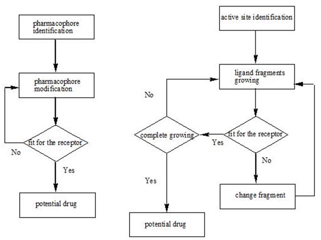
Structure-based drug design (or direct drug design) relies on knowledge of the three dimensional structure of the biological target obtained through methods such as x-ray crystallography or NMR spectroscopy. If an experimental structure of a target is not available, it may be possible to create a homology model of the target based on the experimental structure of a related protein. Using the structure of the biological target, candidate drugs that are predicted to bind with high affinity and selectivity to the target may be designed using interactive graphics and the intuition of a medicinal chemist. Alternatively various automated computational procedures may be used to suggest new drug candidates.
As experimental methods such as X-ray crystallography and NMR develop, the amount of information concerning 3D structures of biomolecular targets has increased dramatically. In parallel, information about the structural dynamics and electronic properties about ligands has also increased. This has encouraged the rapid development of the structure-based drug design. Current methods for structure-based drug design can be divided roughly into two categories. The first category is about “finding” ligands for a given receptor, which is usually referred as database searching. In this case, a large number of potential ligand molecules are screened to find those fitting the binding pocket of the receptor. This method is usually referred as ligand-based drug design. The key advantage of database searching is that it saves synthetic effort to obtain new lead compounds. Another category of structure-based drug design methods is about “building” ligands, which is usually referred as receptor-based drug design. In this case, ligand molecules are built up within the constraints of the binding pocket by assembling small pieces in a stepwise manner. These pieces can be either individual atoms or molecular fragments. The key advantage of such a method is that novel structures, not contained in any database, can be suggested. These techniques are raising much excitement to the drug design community.
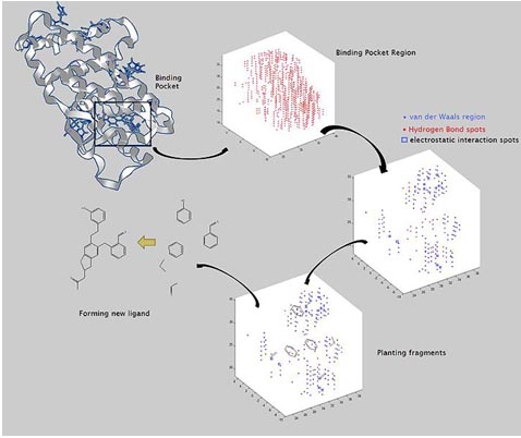
Active site identification is the first step in this program. It analyzes the protein to find the binding pocket, derives key interaction sites within the binding pocket, and then prepares the necessary data for Ligand fragment link. The basic inputs for this step are the 3D structure of the protein and a pre-docked ligand in PDB format, as well as their atomic properties. Both ligand and protein atoms need to be classified and their atomic properties should be defined, basically, into four atomic types:
The space inside the ligand binding region would be studied with virtual probe atoms of the four types above so the chemical environment of all spots in the ligand binding region can be known. Hence we are clear what kind of chemical fragments can be put into their corresponding spots in the ligand binding region of the receptor.
When we want to plant “seeds” into different regions defined by the previous section, we need a fragments database to choose fragments from. The term “fragment” is used here to describe the building blocks used in the construction process. The rationale of this algorithm lies in the fact that organic structures can be decomposed into basic chemical fragments. Although the diversity of organic structures is infinite, the number of basic fragments is rather limited.
Before the first fragment, i.e. the seed, is put into the binding pocket, and add other fragments one by one. we should think some problems. First, the possibility for the fragment combinations is huge. A small perturbation of the previous fragment conformation would cause great difference in the following construction process. At the same time, in order to find the lowest binding energy on the Potential energy surface (PES) between planted fragments and receptor pocket, the scoring function calculation would be done for every step of conformation change of the fragments derived from every type of possible fragments combination. Since this requires a large amount of computation, one may think using other possible strategies to let the program works more efficiently. When a ligand is inserted into the pocket site of a receptor, conformation favor for these groups on the ligand that can bind tightly with receptor should be taken priority. Therefore it allows us to put several seeds at the same time into the regions that have significant interactions with the seeds and adjust their favorite conformation first, and then connect those seeds into a continuous ligand in a manner that make the rest part of the ligand having the lowest energy. The conformations of the pre-placed seeds ensuring the binding affinity decide the manner that ligand would be grown. This strategy reduces calculation burden for the fragment construction efficiently. On the other hand, it reduces the possibility of the combination of fragments, which reduces the number of possible ligands that can be derived from the program. These two strategies above are well used in most structure-based drug design programs. They are described as “Grow” and “Link”. The two strategies are always combined in order to make the construction result more reliable.
In contrast to traditional methods of drug discovery which rely on trial-and-error testing of chemical substances on cultured cells or animals, and matching the apparent effects to treatments, rational drug design begins with a hypothesis that modulation of a specific biological target may have therapeutic value. In order for a biomolecule to be selected as a drug target, two essential pieces of information are required. The first is evidence that modulation of the target will have therapeutic value. This knowledge may come from, for example, disease linkage studies that show an association between mutations in the biological target and certain disease states. The second is that the target is "drugable". This means that it is capable of binding to a small molecule and that its activity can be modulated by the small molecule.
Once a suitable target has been identified, the target is normally cloned and expressed. The expressed target is then used to establish a screening assay. In addition, the three-dimensional structure of the target may be determined.
The search for small molecules that bind to the target is begun by screening libraries of potential drug compounds. This may be done by using the screening assay (a "wet screen"). In addition, if the structure of the target is available, a virtual screen may be performed of candidate drugs. Ideally the candidate drug compounds should be "drug-like", that is they should possess properties that are predicted to lead to oral bioavailability, adequate chemical and metabolic stability, and minimal toxic effects. Several methods are available to estimate druglikeness such Lipinski's Rule of Five and a range of scoring methods such as Lipophilic efficiency. Several methods for predicting drug metabolism have been proposed in the scientific literature, and a recent example is SPORCalc. Due to the complexity of the drug design process, two terms of interest are still serendipity and bounded rationality. Those challenges are caused by the large chemical space describing potential new drugs without side-effects.
Computer-assisted drug design uses computational chemistry to discover, enhance, or study drugs and related biologically active molecules. The most fundamental goal is to predict whether a given molecule will bind to a target and if so how strongly. Molecular mechanics or molecular dynamics are most often used to predict the conformation of the small molecule and to model conformational changes in the biological target that may occur when the small molecule binds to it. Semi-empirical, ab initio quantum chemistry methods, or density functional theory are often used to provide optimized parameters for the molecular mechanics calculations and also provide an estimate of the electronic properties (electrostatic potential, polarizability, etc.) of the drug candidate which will influence binding affinity.
Molecular mechanics methods may also be used to provide semi-quantitative prediction of the binding affinity. Alternatively knowledge based scoring function may be used to provide binding affinity estimates. These methods use linear regression, machine learning, neural nets or other statistical techniques to derive predictive binding affinity equations by fitting experimental affinities to computationally derived interaction energies between the small molecule and the target.
Ideally the computational method should be able to predict affinity before a compound is synthesized and hence in theory only one compound needs to be synthesized. The reality however is that present computational methods provide at best only qualitative accurate estimates of affinity. Therefore in practice it still takes several iterations of design, synthesis, and testing before an optimal molecule is discovered. On the other hand, computational methods have accelerated discovery by reducing the number of iterations required and in addition have often provided more novel small molecule structures.
Drug design with the help of computers may be used at any of the following stages of drug discovery:
In order to overcome the insufficient prediction of binding affinity calculated by recent scoring functions, the protein-ligand interaction and compound 3D structure information are used to analysis. For structure-based drug design, several post-screening analysis focusing on protein-ligand interaction has been developed for improving enrichment and effectively mining potential candidates:
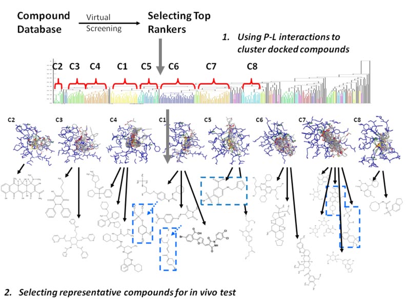
Docking Studies
Docking studies are computational techniques for the exploration of the possible binding modes of a substrate to a given receptor, enzyme or other binding site.
In the field of molecular modeling, docking is a method which predicts the preferred orientation of one molecule to a second when bound to each other to form a stable complex. Knowledge of the preferred orientation in turn may be used to predict the strength of association or binding affinity between two molecules using for example scoring functions.
The associations between biologically relevant molecules such as proteins, nucleic acids, carbohydrates, and lipids play a central role in signal transduction. Furthermore, the relative orientation of the two interacting partners may affect the type of signal produced (e.g., agonism vs antagonism). Therefore docking is useful for predicting both the strength and type of signal produced.
Docking is frequently used to predict the binding orientation of small molecule drug candidates to their protein targets in order to in turn predict the affinity and activity of the small molecule. Hence docking plays an important role in the rational design of drugs. Given the biological and pharmaceutical significance of molecular docking, considerable efforts have been directed towards improving the methods used to predict docking .
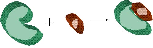
The focus of molecular docking is to computationally simulate the molecular recognition process. The aim of molecular docking is to achieve an optimized conformation for both the protein and ligand and relative orientation between protein and ligand such that the free energy of the overall system is minimized.
Two approaches are particularly popular within the molecular docking community. One approach uses a matching technique that describes the protein and the ligand as complementary surfaces. The second approach simulates the actual docking process in which the ligand-protein pairwise interaction energies are calculated. Both approaches have significant advantages as well as some limitations. These are outlined below.
Geometric matching/ shape complementarity methods describe the protein and ligand as a set of features that make them dockable. These features may include molecular surface/ complementary surface descriptors. In this case, the receptor’s molecular surface is described in terms of its solvent-accessible surface area and the ligand’s molecular surface is described in terms of its matching surface description. The complementarity between the two surfaces amounts to the shape matching description that may help finding the complementary pose of docking the target and the ligand molecules. Another approach is to describe the hydrophobic features of the protein using turns in the main-chain atoms. Yet another approach is to use a Fourier shape descriptor technique. Whereas the shape complementarity based approaches are typically fast and robust, they cannot usually model the movements or dynamic changes in the ligand/ protein conformations accurately, although recent developments allow these methods to investigate ligand flexibility. Shape complementarity methods can quickly scan through several thousand ligands in a matter of seconds and actually figure out whether they can bind at the protein’s active site, and are usually scalable to even protein-protein interactions. They are also much more amenable to pharmacophore based approaches, since they use geometric descriptions of the ligands to find optimal binding.
The simulation of the docking process as such is a much more complicated process. In this approach, the protein and the ligand are separated by some physical distance, and the ligand finds its position into the protein’s active site after a certain number of “moves” in its conformational space. The moves incorporate rigid body transformations such as translations and rotations, as well as internal changes to the ligand’s structure including torsion angle rotations. Each of these moves in the conformation space of the ligand induces a total energetic cost of the system, and hence after every move the total energy of the system is calculated. The obvious advantage of the method is that it is more amenable to incorporate ligand flexibility into its modeling whereas shape complementarity techniques have to use some ingenious methods to incorporate flexibility in ligands. Another advantage is that the process is physically closer to what happens in reality, when the protein and ligand approach each other after molecular recognition. A clear disadvantage of this technique is that it takes longer time to evaluate the optimal pose of binding since they have to explore a rather large energy landscape. However grid-based techniques as well as fast optimization methods have significantly ameliorated these problems.
To perform a docking screen, the first requirement is a structure of the protein of interest. Usually the structure has been determined using a biophysical technique such as x-ray crystallography, or less often, NMR spectroscopy. This protein structure and a database of potential ligands serve as inputs to a docking program. The success of a docking program depends on two components: the search algorithm and the scoring function.
The search space in theory consists of all possible orientations and conformations of the protein paired with the ligand. However in practice with current computational resources, it is impossible to exhaustively explore the search space—this would involve enumerating all possible distortions of each molecule (molecules are dynamic and exist in an ensemble of conformational states) and all possible rotational and translational orientations of the ligand relative to the protein at a given level of granularity. Most docking programs in use account for a flexible ligand, and several attempt to model a flexible protein receptor. Each "snapshot" of the pair is referred to as a pose.
A variety of conformational search strategies have been applied to the ligand and to the receptor. These include:
Conformations of the ligand may be generated in the absence of the receptor and subsequently docked or conformations may be generated on-the-fly in the presence of the receptor binding cavity. Force field energy evaluations are most often used to select energetically reasonable conformations, but knowledge-based methods have also been used.
Computational capacity has increased dramatically over the last decade making possible the use of more sophisticated and computationally intensive methods in computer-assisted drug design. However, dealing with receptor flexibility in docking methodologies is still a thorny issue. The main reason behind this difficulty is the large number of degrees of freedom that have to be considered in this kind of calculations. However, neglecting it, leads to poor docking results in terms of binding pose prediction.
Multiple static structures experimentally determined for the same protein in different conformations are often used to emulate receptor flexibility. Alternatively rotamer libraries of amino acid side chains that surround the binding cavity may be searched to generate alternate but energetically reasonable protein conformations.
The scoring function takes a pose as input and returns a number indicating the likelihood that the pose represents a favorable binding interaction.
Most scoring functions are physics-based molecular mechanics force fields that estimate the energy of the pose; a low (negative) energy indicates a stable system and thus a likely binding interaction. An alternative approach is to derive a statistical potential for interactions from a large database of protein-ligand complexes, such as the Protein Data Bank, and evaluate the fit of the pose according to this inferred potential.
There are a large number of structures from X-ray crystallography for complexes between proteins and high affinity ligands, but comparatively fewer for low affinity ligands as the later complexes tend to be less stable and therefore more difficult to crystallize. Scoring functions trained with this data can dock high affinity ligands correctly, but they will also give plausible docked conformations for ligands that do not bind. This gives a large number of false positive hits, i.e., ligands predicted to bind to the protein that actually don't when placed together in a test tube.
One way to reduce the number of false positives is to recalculate the energy of the top scoring poses using (potentially) more accurate but computationally more intensive techniques such as Generalized Born or Poisson-Boltzmann methods.
A binding interaction between a small molecule ligand and an enzyme protein may result in activation or inhibition of the enzyme. If the protein is a receptor, ligand binding may result in agonism or antagonism. Docking is most commonly used in the field of drug design — most drugs are small organic molecules, and docking may be applied to:
Protein Structure
Proteins are an important class of biological macromolecules present in all organisms. All proteins are polymers of amino acids. Classified by their physical size, proteins are nanoparticles (definition: 1–100 nm). Each protein polymer – also known as a polypeptide – consists of a sequence of 20 different L-α-amino acids, also referred to as residues. For chains under 40 residues the term peptide is frequently used instead of protein. To be able to perform their biological function, proteins fold into one or more specific spatial conformations, driven by a number of non-covalent interactions such as hydrogen bonding, ionic interactions, Van Der Waals forces, and hydrophobic packing. To understand the functions of proteins at a molecular level, it is often necessary to determine their three-dimensional structure. This is the topic of the scientific field of structural biology, which employs techniques such as X-ray crystallography, NMR spectroscopy, and dual polarisation interferometry to determine the structure of proteins.
Protein structures range in size from tens to several thousand residues. Very large aggregates can be formed from protein subunits: for example, many thousand actin molecules assemble into a microfilament.
A protein may undergo reversible structural changes in performing its biological function. The alternative structures of the same protein are referred to as different conformations, and transitions between them are called conformational changes.
The primary structure refers to the sequence of the different amino acids of the peptide or protein. The primary structure is held together by covalent or peptide bonds, which are made during the process of protein biosynthesis or translation. The two ends of the polypeptide chain are referred to as the carboxyl terminus (C-terminus) and the amino terminus (N-terminus) based on the nature of the free group on each extremity. Counting of residues always starts at the N-terminal end (NH2-group), which is the end where the amino group is not involved in a peptide bond. The primary structure of a protein is determined by the gene corresponding to the protein. A specific sequence of nucleotides in DNA is transcribed into mRNA, which is read by the ribosome in a process called translation. The sequence of a protein is unique to that protein, and defines the structure and function of the protein. The sequence of a protein can be determined by methods such as Edman degradation or tandem mass spectrometry. Often however, it is read directly from the sequence of the gene using the genetic code. Post-translational modifications such as disulfide formation, phosphorylations and glycosylations are usually also considered a part of the primary structure, and cannot be read from the gene.
Secondary structure refers to highly regular local sub-structures. Two main types of secondary structure, the alpha helix and the beta strand, were suggested in 1951 by Linus Pauling and coworkers. These secondary structures are defined by patterns of hydrogen bonds between the main-chain peptide groups. They have a regular geometry, being constrained to specific values of the dihedral angles ψ and φ on the Ramachandran plot. Both the alpha helix and the beta-sheet represent a way of saturating all the hydrogen bond donors and acceptors in the peptide backbone. Some parts of the protein are ordered but do not form any regular structures. They should not be confused with random coil, an unfolded polypeptide chain lacking any fixed three-dimensional structure. Several sequential secondary structures may form a "supersecondary unit".
Tertiary structure refers to three-dimensional structure of a single protein molecule. The alpha-helices and beta-sheets are folded into a compact globule. The folding is driven by the non-specific hydrophobic interactions (the burial of hydrophobic residues from water), but the structure is stable only when the parts of a protein domain are locked into place by specific tertiary interactions, such as salt bridges, hydrogen bonds, and the tight packing of side chains and disulfide bonds. The disulfide bonds are extremely rare in cytosolic proteins, since the cytosol is generally a reducing environment.
Quaternary structure is a larger assembly of several protein molecules or polypeptide chains, usually called subunits in this context. The quaternary structure is stabilized by the same non-covalent interactions and disulfide bonds as the tertiary structure. Complexes of two or more polypeptides (i.e. multiple subunits) are called multimers. Specifically it would be called a dimer if it contains two subunits, a trimer if it contains three subunits, and a tetramer if it contains four subunits. The subunits are frequently related to one another by symmetry operations, such as a 2-fold axis in a dimer. Multimers made up of identical subunits are referred to with a prefix of "homo-" (e.g. a homotetramer) and those made up of different subunits are referred to with a prefix of "hetero-" (e.g. a heterotetramer, such as the two alpha and two beta chains of hemoglobin). Many proteins do not have the quaternary structure and function as monomers.
Proteins are frequently described as consisting from several structural units.
Despite the fact that there are about 100,000 different proteins expressed in eukaryotic systems, there are many fewer different domains, structural motifs and folds. This is partly a consequence of evolution, since genes or parts of genes can be doubled or moved around within the genome. This means that, for example, a protein domain might be moved from one protein to another thus giving the protein a new function. Because of these mechanisms, pathways and mechanisms tend to be reused in several different proteins.
A Ramachandran plot (also known as a Ramachandran map or a Ramachandran diagram or a [φ,ψ] plot), developed by Gopalasamudram Narayana Ramachandran and Viswanathan Sasisekharan is a way to visualize dihedral angles ψ against φ of amino acid residues in protein structure. It shows the possible conformations of ψ and φ angles for a polypeptide.
Mathematically, the Ramachandran plot is the visualization of a function f: (-p, +p) X (-p + +p) -> R+. The domain of this function is the torus. Hence, the conventional Ramachandran plot is a projection of the torus on the plane, resulting in a distorted view and the presence of discontinuities.
One would expect that larger side chains would result in more restrictions and consequently a smaller allowable region in the Ramachandran plot. In practice this does not appear to be the case; only the methylene group at the α position has an influence. Glycine has a hydrogen atom, with a smaller van der Waals radius, instead of a methyl group at the α position. Hence it is least restricted and this is apparent in the Ramachandran plot for glycine for which the allowable area is considerably larger.
In contrast, the Ramachandran plot for proline shows only a very limited number of possible combinations of ψ and φ.
The Ramachandran plot was calculated just before the first protein structures at atomic resolution were determined. Forty years later there were tens of thousands of high-resolution protein structures determined by X-ray crystallography and deposited in the Protein Data Bank (PDB). From one thousand different protein chains, Ramachandran plots of over 200 000 amino acids were plotted, showing some significant differences, especially for glycine (Hovmöller et al., 2002). The upper left region was found to be split into two; one to the left containing amino acids in beta sheets and one to the right containing the amino acids in random coil of this conformation.
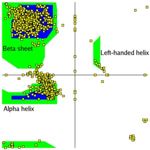
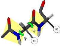
One can also plot the dihedral angles in polysaccharides and other polymers in this fashion. For the first two protein side-chain dihedral angles a similar plot is the Janin Plot.
Protein structure comparison
With the visualization and computer graphics tools available, it becomes easy to observe and compare protein structures. To compare protein structures is to analyze two or more protein structures for similarity. The comparative analysis often, but not always, involves the direct alignment and superimposition of structures in a three-dimensional space to reveal which part of structure is conserved and which part is different at the three-dimensional level.
This structure comparison is one of the fundamental techniques in protein structure analysis. The comparative approach is important in finding remote protein homologs. Because protein structures have a much higher degree of conservation than the sequences, proteins can share common structures even without sequence similarity. Thus, structure comparison can often reveal distant evolutionary relationships between proteins, which is not feasible using the sequence-based alignment approach alone. In addition, protein structure comparison is a prerequisite for protein structural classification into different fold classes. It is also useful in evaluating protein prediction methods by comparing theoretically predicted structures with experimentally determined ones. One can always compare structures manually or by eye, which is often practiced.
However, the best approach is to use computer algorithms to automate the task and thereby get more accurate results. Structure comparison algorithms all employ scoring schemes to measure structural similarities and to maximize the structural similarities measured using various criteria. The algorithmic approaches to comparing protein geometric properties can be divided into three categories: the first superposes protein structures by minimizing intermolecular distances; the second relies on measuring intramolecular distances of a structure; and the third includes algorithms that combine both intermolecular and intramolecular approaches.
Intermolecular Method
The intermolecular approach is normally applied to relatively similar structures. To compare and superpose two protein structures, one of the structures has to be moved with respect to the other in such a way that the two structures have a maximum overlap in a three-dimensional space. This procedure starts with identifying equivalent residues or atoms. After residue–residue correspondence is established, one of the structures is moved laterally and vertically toward the other structure, a process known as translation, to allow the two structures to be in the same location (or same coordinate frame). The structures are further rotated relative to each other around the three-dimensional axes, during which process the distances between equivalent positions are constantly measured. The rotation continues until the shortest intermolecular distance is reached. At this point, an optimal superimposition of the two structures is reached. After superimposition, equivalent residue pairs can be identified, which helps to quantitate the fitting between the two structures.
An important measurement of the structure fit during superposition is the distance between equivalent positions on the protein structures. This requires using a leastsquare-fitting function called root mean square deviation (RMSD), which is the square root of the averaged sum of the squared differences of the atomic distances.
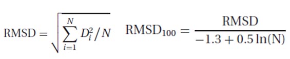
where D is the distance between coordinate data points and N is the total number of corresponding residue pairs. In practice, only the distances between Cα carbons of corresponding residues are measured. The goal of structural comparison is to achieve a minimum RMSD. However, the problem with RMSD is that it depends on the size of the proteins being compared. For the same degree of sequence identity, large proteins tend to have higher RMSD values than small proteins when an optimal alignment is reached. Recently, a logarithmic factor has been proposed to correct this size-dependency problem. This new measure is called RMSD100 and is determined by the following formula in the figure. Where N is the total number of corresponding atoms. Although this corrected RMSD is more reliable than the raw RMSD for structure superposition, a low RMSD value by no means guarantees a correct alignment or an alignment with biological meaning. Careful scrutiny of the automatic alignment results is always recommended.
The most challenging part of using the intermolecular method is to identify equivalent residues in the first place, which often resorts to sequence alignment methods. Obviously, this restricts the usefulness of structural comparison between distant homologs.
A number of solutions have been proposed to compare more distantly related structures. One approach that has been proposed is to delete sequence variable regions outside secondary structure elements to reduce the search time required to find an optimum superposition. However, this method does not guarantee an optimal alignment. Another approach adopted by some researchers is to divide the proteins into small fragments (e.g., every six to nine residues). Matching of similar regions at the three-dimensional level is then done fragment by fragment. After finding the best fitting fragments, a joint superposition for the entire structure is performed. The third approach is termed iterative optimization, during which the two sequences are first aligned using dynamic programming. Identified equivalent residues are used to guide a first round of superposition. After superposition, more residues are identified to be in close proximity at the three-dimensional level and considered as equivalent residues. Based on the newly identified equivalent residues, a new round of superposition is generated to refine from the previous alignment. This procedure is repeated until the RMSD values cannot be further improved.
Intramolecular Method
The intramolecular approach relies on structural internal statistics and therefore does not depend on sequence similarity between the proteins to be compared. In addition, this method does not generate a physical superposition of structures, but instead provides a quantitative evaluation of the structural similarity between corresponding residue pairs. The method works by generating a distance matrix between residues of the same protein. In comparing two protein structures, the distance matrices from the two structures are moved relative to each other to achieve maximum overlaps. By overlaying two distance matrices, similar intramolecular distance patterns representing similar structure folding regions can be identified. For the ease of comparison, each matrix is decomposed into smaller submatrices consisting of hexapeptide fragments. To maximize the similarity regions between two structures, a Monte Carlo procedure is used. By reducing three-dimensional information into two-dimensional information, this strategy identifies overall structural resemblances and common structure cores.
Combined method
A recent development in structure comparison involves combining both inter- and intramolecular approaches. In the hybrid approach, corresponding residues can be identified using the intramolecular method. Subsequent structure superposition can be performed based on residue equivalent relationships. In addition to using RMSD as a measure during alignment, additional structural properties such as secondary structure types, torsion angles, accessibility, and local hydrogen bonding environment can be used. Dynamic programming is often employed to maximize overlaps in both inter- and intramolecular comparisons.
Multiple structure alignment
In addition to pairwise alignment, a number of algorithms can also perform multiple structure alignment. The alignment strategy is similar to the Clustal sequence alignment using a progressive approach (see Chapter 5). That is, all structures are first compared in a pairwise fashion. A distance matrix is developed based on structure similarity scores such as RMSD. This allows construction of a phylogenetic tree, which guides the subsequent clustering of the structures. The most similar two structures are then realigned. The aligned structures create a median structure that allows other structures to be progressively added for comparison based on the hierarchy described in the guide tree. When all the structures in the set are added, this eventually creates a multiple structure alignment. Several popular on-line structure comparison resources are discussed next.
DALI (www2.ebi.ac.uk/dali/) is a structure comparison web server that uses the intramolecular distance method. It works by maximizing the similarity of two distance graphs. The matrices are based on distances between all Cα atoms for each individual protein. Two distance matrices are overlaid and moved one relative to the other to identify most similar regions. DALI uses a statistical significance value called aZ-score to evaluate structural alignment. The Z-score is the number of standard deviations from the average score derived from the database background distribution. The higher the Z-score when comparing a pair of protein structures, the less likely the similarity observed is a result of random chance. Empirically, a Z-score>4 indicates a significant level of structure similarity. The web server is at the same time a database that contains Z-scores of all precomputed structure pairs of proteins in PDB. The user can upload a structure to compare it with all known structures, or performa pairwise comparison of two uploaded structures.
CE (Combinatorial Extension; http://cl.sdsc.edu/ce.html) is a web-based program that also uses the intramolecular distance approach. However, unlike DALI, a type of heuristics is used. In this method, every eight residues are treated as a single residue. The Cα distance matrices are constructed at the level of octameric “residues.” In this way, the computational time required to search for the best alignment is considerably reduced, at the expense of alignment accuracy. CE also uses a Z-score as a measure of significance of an alignment. A Z-score >3.5 indicates a similar fold.
VAST (Vector Alignment Search Tool; www.ncbi.nlm.nih.gov:80/Structure/VAST/vast.shtml) is a web server that performs alignment using both the inter- and intramolecular approaches. The superposition is based on information of directionality of secondary structural elements (represented as vectors). Optimal alignment between two structures is defined by the highest degree of vector matches.
SSAP (www.biochem.ucl.ac.uk/cgi-bin/cath/GetSsapRasmol.pl) is a web server that uses an intramolecular distance–based method in which matrices are built based on the Cβ distances of all residue pairs. When comparing two different matrices, a dynamic programming approach is used to find the path of residue positions with optimal scores. The dynamic programming is applied at two levels, one at a lower level in which all residue pairs between the proteins are compared and another at an upper level in which subsequently identified equivalent residue pairs are processed to refine the matching positions. This process is known as double dynamic programming. An SSAP score is reported for structural similarity. A score above 70 indicates a good structural similarity.
STAMP (www.compbio.dundee.ac.uk/Software/Stamp/stamp.html) is a UNIX program that uses the intermolecular approach to generate protein structure alignment. The main feature is the use of iterative alignment based on dynamic programming to obtain the best superposition of two or more structures.
Protein Structure Visualization
The main feature of computer visualization programs is interactivity, which allows users to visually manipulate the structural images through a graphical user interface. At the touch of a mouse button, a user can move, rotate, and zoom an atomic model on a computer screen in real time, or examine any portion of the structure in great detail, as well as draw it in various forms in different colors. Further manipulations can include changing the conformation of a structure by protein modeling or matching a ligand to an enzyme active site through docking exercises. Because a Protein Data Bank (PDB) data file for a protein structure contains only x, y, and z coordinates of atoms (see Chapter 12), the most basic requirement for a visualization program is to build connectivity between atoms to make a view of a molecule. The visualization program should also be able to produce molecular structures in different styles, which include wire frames, balls and sticks, space-filling spheres, and ribbons (Fig.).
A wire-frame diagram is a line drawing representing bonds between atoms. The wire frame is the simplest form of model representation and is useful for localizing positions of specific residues in a protein structure, or for displaying a skeletal form of a structure when Cα atoms of each residue are connected. Balls and sticks are solid spheres and rods, representing atoms and bonds, respectively. These diagrams can also be used to represent the backbone of a structure. In a space-filling representation (or Corey, Pauling, and Koltan [CPK]), each atom is described using large solid spheres with radii corresponding to the van der Waals radii of the atoms. Ribbon diagrams use cylinders or spiral ribbons to represent α-helices and broad, flat arrows to represent β-strands. This type of representation is very attractive in that it allows easy identification of secondary structure elements and gives a clear view of the overall topology of the structure. The resulting images are also visually appealing.
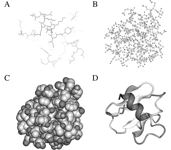
Examples of molecular structure visualization forms. (A) Wireframes. (B) Balls and sticks.
(C) Space-filling spheres. (D) Ribbons
Different representation styles can be used in combination to highlight a certain feature of a structure while deemphasizing the structures surrounding it. For example, a cofactor of an enzyme can be shown as space-filling spheres while the rest of the protein structure is shown as wire frames or ribbons. Some widely used and freely available software programs for molecular graphics are introduced next with examples of rendering provided in Figure.
RasMol (http://rutgers.rcsb.org/pdb/help-graphics.html#rasmol download) is a command-line–based viewing program that calculates connectivity of a coordinate file and displays wireframe, cylinder, stick bonds, α-carbon trace, space-filling (CPK) spheres, and ribbons. It reads both PDB and mmCIF formats and can display a whole molecule or specific parts of it. It is available in multiple platforms: UNIX, Windows, and Mac. RasTop (www.geneinfinity.org/rastop/) is a new version of RasMol for Windows with a more enhanced user interface.
Swiss-PDBViewer (www.expasy.ch/spdbv/) is a structure viewer for multiple platforms. It is essentially a Swiss-Army knife for structure visualization and modeling because it incorporates so many functions in a small shareware program. It is capable of structure visualization, analysis, and homology modeling. It allows display of multiple structures at the same time in different styles, by charge distribution, or by surface accessibility. It can measure distances, angles, and even mutate residues. In addition, it can calculate molecular surface, electrostatic potential, Ramachandran plot, and so on. The homology modeling part includes energy minimization and loop modeling.
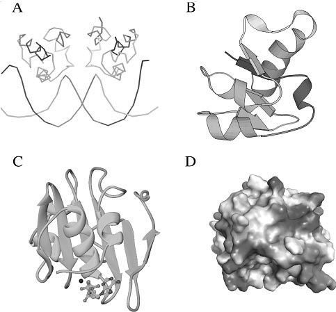
Examples of molecular graphic generated by (A) Rasmol, (B) Molscript, (C) Ribbons, and
(D) Grasp
Molscript (www.avatar.se/molscript/) is a UNIX program capable of generating wire-frame, space-filling, or ball-and-stick styles. In particular, secondary structure elements can be drawn with solid spirals and arrows representing α-helices and β-strands, respectively. Visually appealing images can be generated that are of publication quality. The drawback is that the program is command-line–based and not very user friendly. A modified UNIX program called Bobscript (www.strubi.ox.ac.uk/bobscript/) is available with enhanced features.
Ribbons (http://sgce.cbse.uab.edu/ribbons/) another UNIX program similar to Molscript, generates ribbon diagrams depicting protein secondary structures. Aesthetically appealing images can be produced that are of publication quality.However, the program, which is also command-line-based, is extremely difficult to use.
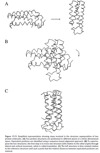
Grasp (http://trantor.bioc.columbia.edu/grasp/) is a UNIX program that generates solid molecular surface images and uses a gradated coloring scheme to display electrostatic charges on the surface. There are also a number of web-based visualization tools that use Java applets. These programs tend to have limited molecular display features and low-quality images. However, the advantage is that the user does not have to download, compile, and install the programs locally, but simply view the structures on a web browser using any kind of computer operating system. In fact, the PDB also attempts to simplify the database structure display for end users. It has incorporated a number of light-weight Java-based structure viewers in the PDB web site.
WebMol (www.cmpharm.ucsf.edu/cgi-bin/webmol.pl) is a web-based program built based on a modified RasMol code and thus shares many similarities with RasMol. It runs directly on a browser of any type as an applet and is able to display simple line drawing models of protein structures. It also has a feature of interactively displaying
Ramachandran plots for structure model evaluation.
Chime (www.mdlchime.com/chime/) is ap lug-in for web browsers; it isnot a standalone program and has to be invoked in a web browser. The program is also derived from RasMol and allows interactive display of graphics of protein structures inside a web browser.
Cn3D (www.ncbi.nlm.nih.gov/Structure/CN3D/cn3d.shtml) is a helper application for web browsers to display structures in the MMDB format from the NCBI’s structural database. It can be used on- or offline as a stand-alone program. It is able to render three-dimensional molecular models and display secondary structure cartoons. The drawback is that it does not recognize the PDB format.
CONFORMATIONAL ENERGY CALCULATIONS AND MOLECULAR DYNAMICS
One of the main goals of conformational energy calculations on polypeptides and proteins is the analysis and prediction of their three-dimensional structures. These structures are the result of the balance of intra- and intermolecular interactions, which in turn can be expressed in terms of interatomic potential energy functions. In order to gain an understanding of the physical reasons for the folded structures of these molecules, it is necessary to elucidate how the potential energy determines the structures themselves, their stability, and their dynamic properties.
A protein is a collection of atoms. The interactions between the atoms create a unique state of maximum stability. The computational difficulties in this approach arise because (a) the model of the interatomic interactions is not complete or exact, and (b) even if the model were exact we should face an optimization problem in a large number of variables, involving nonlinearities in the objective function and the constraints, creating a very rough energy surface with many local minima. Like a golf course with many bunkers, such problems are very difficult.
The interactions between atoms in a molecule can be divided into:
a. primary chemical bonds - strong interactions between atoms that must be close together in space. These are regarded as a fixed set of interactions that are not broken or formed when the conformation of a protein changes, but are equally consistent with a large number of conformations.
b. weaker interactions that depend on the conformation of the chain. These can be significant in some conformations and not in others - they affect sets of atoms that are brought into proximity by different folds of the chain.
The conformation of a protein can be specified by giving the list of atoms in the structure, their coordinates, and the set of primary chemical bonds between them (this can be read off, with only slight ambiguity, from the amino acid sequence). Terms used in the evaluation of the energy of a conformation typically include
Bond stretching: Σbonds Kr(r - r0)2. Here r0 is the equilibrium interatomic separation and Kr is the force constant for stretching the bond. r0 and Kr depend on the type of chemical bond.
Bond angle bend: Σangles Kθ (θ - θ0)2. For any atom i that is chemically bonded to two (or more) other atoms j and k, the angle i - j - k has an equilibrium value θ 0 and a force constant for bending Kθ.
Other terms to enforce proper stereochemistry penalize deviations from planarity of certain groups, or enforce correct chirality (handedness) at certain centres.
Torsion angle: Σdihedrals 1/2 Vn[1 + cos nφ ]. For any four connected atoms: i bonded to j bonded to k bonded to l, the energy barrier to rotation of atom l with respect to atom i around the j - k bond is given by a periodic potential. Vn is the height of the barrier to internal rotation; n barriers are encountered during a full 360° rotation. The mainchain conformational angles φ ,
ψ , and ω are examples of torsional rotations.
Van der Waals interactions: ΣiΣj<i(AijRij-12 - BijRij-6) For each pair of non-bonded atoms i and j, the first term accounts for a short-range repulsion and the second term for a long-range attraction between them. The parameters A and B depend on atom type. Rij is the distance between atoms i and j.
Hydrogen bond: ΣiΣj<i(CijRij-12 - DijRij-10) The hydrogen bond is a weak chemical/electrostatic interaction between two polar atoms. Its strength depends on distance and also on the bond angle. This approximate hydrogen bond potential does not explicitly reflect the angular dependence of hydrogen bond strength; other potentials attempt to account for hydrogen bond geometry more accurately.
Electrostatics: ΣiΣj<iQiQj/(εRij). Qi and Qj are the effective charges on the atoms, Rij is the distance between them, and ∈ is the dielectric 'constant'. This formula applies only approximately to media that are not infinite and isotropic, including proteins.
Solvent: Interactions with the solvent, water, and cosolutes such as salts and sugars, are crucial for the thermodynamics of protein structures. Attempts to model the solvent as a continuous medium, characterized primarily by a dielectric constant, are approximations. With the increase in available computer power, it is now possible to include solvent explicitly, simulating the motion of a protein in a box of water molecules.
There are numerous sets of conformational energy potentials of this or closely related forms, and a great deal of effort has gone into the tuning of parameter sets. The energy of a conformation is computed by summing these terms over all appropriate sets of interacting atoms.
The potential functions satisfy necessary but not sufficient conditions for successful structure prediction. One test is to take the right answer - an experimentally determined protein structure - as a starting conformation, and minimize the energy starting from there. In general most energy functions produce a minimized conformation that is about 1 Å(root-mean-square deviation) away from the starting model. This can be thought of as a measure of the resolution of the force field. Another test has been to take deliberately misfolded proteins and minimize their conformational energies, to see whether the energy value of the local minimum in the vicinity of the correct fold is significantly lower than that of the local minimum in the vicinity of an incorrect fold. Such tests reveal that multiple local minima cannot be reliably distinguished from the correct one on the basis of calculated conformational energies.
Attempts to predict the conformation of a protein by minimization of the conformational energy have so far not provided a method for predicting protein structure from amino acid sequence. In order to overcome the problems both of getting trapped in local minima, and of the absence of a good model for protein-solvent interactions, molecular dynamics models have been developed. The protein plus explicit solvent molecules are treated - via the force field - by classical Newtonian mechanics. It is true that this permits exploration of a much larger sector of phase space. However, as an a priori method of structure prediction, it has still not succeeded consistently. However, these are calculations that are extremely computationally intensive and here, perhaps more than anywhere else in this field, advances deriving from the increased 'brute force' power of processors will have an effect.
In the meantime, molecular dynamics, if supplemented by experimental data, regularly makes extremely important contributions to structure determinations by both X-ray crystallography usually) and nuclear magnetic resonance (always). How is molecular dynamics integrated into the process of structure determination? For any conformation, one can measure the consistency of the model with the experimental data. In the case of crystallography, the experimental data are the absolute values of the Fourier transform of the electron density of the molecule. In the case of nuclear magnetic resonance, the experimental data provide constraints on the distances between certain pairs of residues. But in both X-ray crystallography and nuclear magnetic resonance, the experimental data underdetermine the protein structure. To solve a structure one must seek a set of coordinates that minimizes a combination of the deviation from the experimental data and the conformational energy. Molecular dynamics is successful at determining such coordinate sets: the dynamics provides adequate coverage of conformation space, and the bias derived from the experimental data channels the calculation towards the correct structure.
MOLECULAR INTERACTIONS
The molecular associations/interactions are the basis of transformation and regulation of genetic information and all cellular actions and biochemical reactions, such as cell-cell recognition, neuronal signaling, hormonal action, and protein and enzyme functions. Central to such molecular-molecular associations/interactions are protein-nucleic, protein-carbohydrate, and protein-lipid interactions.
DNA-PROTEIN INTERACTION
Molecular interactions/associations are governed by–
(a) The size and shape of the ligand that imposes steric hindrance.
(b) Electronic potential at the site of interaction.
Molecular interactions that occur in protein-nucleic acid complexes are between
(i) Protein side chains and DNA backbone (50%).
(ii) Protein side chains and DNA side chains (30%).
(iii) Protein backbone and DNA backbone.
(iv) Protein backbone and DNA side chain (1%).
These types of interactions can also serve as general types of interactions in all macromolecular associations. The interactions can be non-specific, such as those found in histone-DNA association in chromatin, as well as specific as found in restriction endonuclease-DNA complexes. While non-specific interactions enable docking of the interacting molecular moieties, the specific interactions enable sequence-specific associations. Molecular interactions between functional groups can be classified under (1) electrostatic, (2) hydrogen bonding and (3) intercalation interactions.
Electrostatic Interactions
Electrostatic interactions in protein-nucleic acid complexes occur between positively charged side chains of proteins (e.g. lysyl, arginyl) and negatively charged phosphate groups of the nucleic acid backbone. Electrostatic interactions are also mediated by metal ions. Electrostatic potential of the basepair moiety plays an important role in protein-nucleic acid interactions in the major and minor grooves.
Sequence-specific hydrogen bonding
Sequence-specific interactions between proteins and nucleic acids are largelyo via hydrogen bons, between nucleic acid side chains and parts of nucleic acid base can act as aceptors as well as donors of hydrogen bonds. As the hydrogen bonds have directionality, the specificity is imparted in hydrogen bond networks that involve two or more hydrogen bonds (oligodentate hydrogen bond network). Such oligodentate hydrogen bond networks are the fundamental features of sequence-specific interactions between nucleoproteins and nucleic acids in spatial and temporal regulation and transmission of genetic information (e.g. DNA-regulatory proteins, restriction enzymes).
Interaction
Hydrophobic interactions are not directional. However, intercalation (stacking of planar moieties) is a special case of hydrophobic interactions that impart directionality. Interaction plays a crucial role in structure stability and function in nucleic acids and protein-nucleic acids complexes. While storage of genetic information in nucleic acids is by Watson-Crick type base pairs, such planar hydrogen-bond networks would not have been possible without proper base stacking.
In protein-nucleic acid complexes, the aromatic side chains, such as Phe, Trp and Tyr can interact in the major and minor grooves of nucleic acids by intercalation and further stabilized by hydrogen bonding between the peptide and nucleic acid moieties. Such a combination of intercalation and hydrogen bonding imparts specificity in protein-nucleic acid interactions.
DNA-regulatory Proteins
DNA-regulatory proteins are associated with transcriptional control. These proteins bind to specific DNA sequences and thus help in switching on or off genetic coding as required. Most of these proteins bind in the major groove of the DNA. Many of them have an ordered organization of secondary structures (super-secondary structures) that form distinct structural motifs (e.g. helix-turn-helix, zinc-finger and leucine-zipper motifs).
“Helix-turn-Helix” Motif”
Many of the prokaryotic transcriptional regulatory proteins have the helix-turn-helix (HTH)structural motif. The HTH motif is approximately 20 residues long, with a 7-residue helix, a short turn, and nine-residue helix (recognition helix). The ‘recognition helix’ fits into the major groove of B-DNA. The specificities of the various helix-turn-helix motifs for binding to different DNA sequences arise primarily from the different amino acid side chains that emanate for the “recognition helix”. The other helix lies across the major groove and makes non-specific contacts with DNA.
“Zinc-finger” Motifs
Several types of zinc-finger motifs have been identified. In these the Zn2+ ion forms a coordination moiety (moieties) with Cys/His residues of the protein. Zinc-finger motifs are found not only in DNA-binding proteins but in proteins in general, involving protein-protein interactions.
“Leucine-zipper” Motif
The leucine-zipper motif has been found in several eukaryotic transcriptional regulatory proteins. The motif (~ 30 amino acid residues) consists of leu or ile at seven residue intervals (heptad spacing). The basic motif is (–L–X6–L–X6–L–X6–X6–L–X6–).
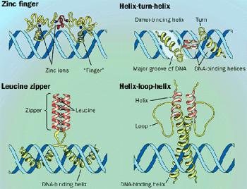
PROTEIN-PROTEIN INTERACTIONS
Protein-protein interactions include biological pathways, regulatory systems and signaling cascades. They play a major role in almost all relevant physiological processes occurring in living organisms, including DNA replication and transcription, RNA splicing, protein biosynthesis, and signal transduction. Molecular interactions that occur in protein-nucleic acid complexes are the same that occur between protein-protein interactions/associations, namely non-bonded interactions– ionic, hydrogen bonding, van der Waals, and hydrophobic interactions. Structure-function aspects can be determined by X-ray crystallography and NME spectroscopy. Physicochemical and biomolecular methods are– phage display, protein arrays, immunoprecipitation assays, and yeast two-hybrids (screening technique to identify genes encoding interacting proteins). Yeast two hybrid is an approach to studying protein-protein interactions. The basic format involves the creation of two hybrid molecules, one in which a “bait” protein is fused with a transcription factor, and one in which a “prey” protein is fused with a related transcription factor. If the bait and prey proteins indeed interact, then the two factors fused to these two proteins are also brought into proximity with each other. As a result, a specific signal is produced, indicating an interaction has taken place. Yeast three hybrid: Modification of yeast two hybrid system. The third hybrid may be a first one with a RNA or with a small molecule that is a cell permeable chemical inducer of dimerization. The three-hybrid system enables the detection of RNA-protein interactions in yeast using simple phenotypic assays.
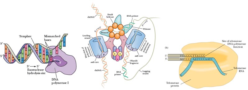
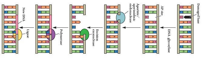
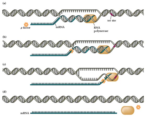
PROTEIN-CARBOHYDRATE INTERACTIONS
Many proteins covalently conjugated with carbohydrates by post-translational modification. These proteins, called glycoproteins, are classified as O-linked if the sugars are attached to the –OH groups of serine or threonine, and as N-linked if the sugars are attached to the amide nitrogen of the asparagine side chain. Glycoproteins are involved wide variety of biological functions. For example, the variability in the composition of the carbohydrate moieties of glycoproteins of erythrocytes that determine the blood groups specificity. Carbohydrates of glycoproteins appear to act as recognition markers in various cellular processes.
Proteoglycans are a family of glycoproteins whose carbohydrate moieties are predominantly glycosaminoglycans. The structures of only a few proteoglycans are known, and even these few display considerable diversity (Figure 7.36). Those known range in size from serglycin, having 104 amino acid residues (10.2 kD), to versican, having 2409 residues (265 kD). Each of these proteoglycans contains one or two types of covalently linked glycosaminoglycans. In the known proteoglycans, the glycosaminoglycan units are O-linked to serine residues of Ser-Gly dipeptide sequences. Serglycin is named for a unique central domain of 49 amino acids composed of alternating serine and glycine residues. The cartilage matrix proteoglycan contains 117 Ser-Gly pairs to which chondroitin sulfates attach. Decorin, a small proteoglycan secreted by fibroblasts and found in the extracellular matrix of connective tissues, contains only three Ser-Gly pairs, only one of which is normally glycosylated. In addition to glycosaminoglycan units, proteoglycans may also contain other N-linked and O-linked oligosaccharide groups.
The oligosaccharides attached to glycoproteins serve various functions. For example, some proteins require N-linked oligosaccharides in order to fold properly in the ER. This function has been demonstrated in studies with the antibiotic tunicamycin, which blocks the first step in formation of thedolichol-linked precursor of N-linked oligosaccharides . In the presence of tunicamycin, for instance, the hemagglutinin precursor polypeptide (HA0) is synthesized, but it cannot fold properly and form a normal trimer; in this case, the protein remains, misfolded, in the rough ER. Moreover, mutation in the HA sequence of just one asparagine that normally is glycosylated to a glutamine residue, thereby preventing addition of an N-linked oligosaccharide to that site, causes the protein to accumulate in the ER in an unfolded state.
In addition to promoting proper folding, N-linked oligosaccharides also confer stability on many secreted gly-coproteins. Many secretory proteins fold properly and are transported to their final destination even if the addition of all N-linked oligosaccharides is blocked, for example, by tunicamycin. However, such nonglycosylated proteins have been shown to be less stable than their glycosylated forms. For instance, glycosylated fibronectin, a normal component of the extracellular matrix, is degraded much more slowly by tissue proteases than is nonglycosylated fibronectin. Oligosaccharides on certain cell-surface glycoproteins also play a role in cell-cell adhesion. For example, the plasma membrane of white blood cells (leukocytes) contains celladhesion molecules (CAMs) that are extensively glycosylated.
The oligosaccharides in these molecules interact with a sugar-binding domain in certain CAMs found on endothelial cells lining blood vessels. This interaction tethers the leukocytes to the endothelium and assists in their movement into tissues during an inflammatory response to infection. Other cell-surface glycoproteins possess oligosaccharide side chains that can induce an immune response. A common example is the A, B, O blood-group antigens, which are O-linked oligosaccharides attached to glycoproteins and glycolipids on the surface of erythrocytes and other cell types.
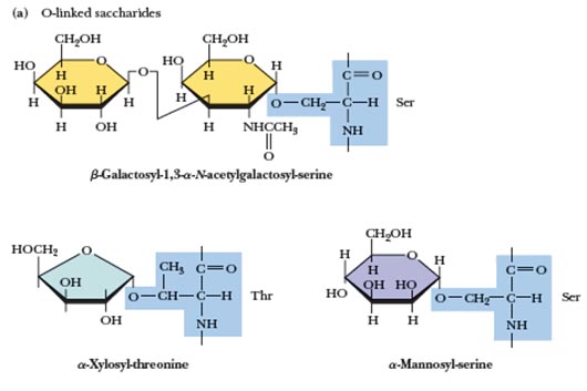
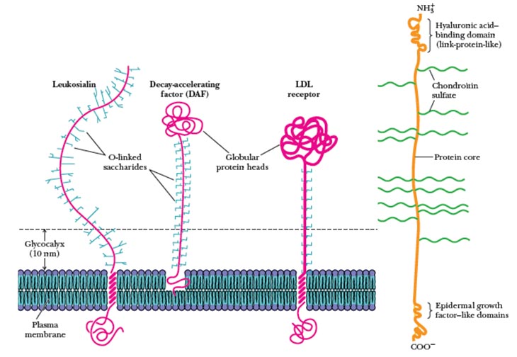
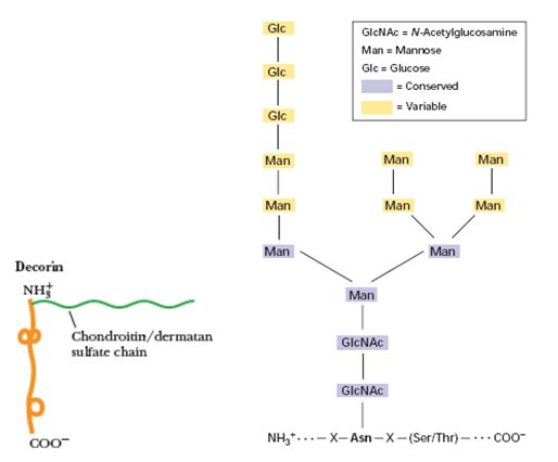
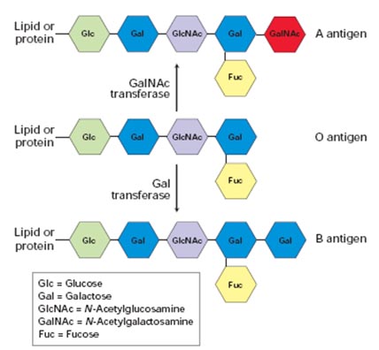
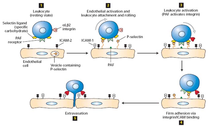
PROTEIN-LIPID INTERACTIONS
Protein-lipid interactions are predominantly hydrophobic in character. The major function of lipoproteins is to aid in the storage transport of lipid and cholesterol.
DNA – MOLECULE INTERACTION
DNA is an extremely long molecule, so long in fact that it would not fit into the nucleus of the cell if it existed as a linear molecule. It has to be coiled into a more compact three dimentional shape which can fit into the nucleus – a process known as supercoiling. This process requires the action of a family of enzymes called topoisomerases. Inhibition of these enzymes can efficiently block transcription and replication. Therefore cleavage of supercoiled DNA into nicked circular and linear forms also are necessary to block these processes. Another important property of DNA is its ability to interact reversibly with a broad range of chemical species that include water, metal ions and their complexes, small organic molecules and proteins. Because of their relative simplicity, the interactions of small molecules with nucleic acids have provided accurate information about nucleic acid binding specificity. Incidentally, this specificity differentiates between two types of DNA cleavage i.e. oxidative and hydrolytic.
Molecules and ions interact with DNA in three primary ways which are significantly different:
a. binding along the exterior of the helix through interactions which are generally non-specific and are primarily electrostatic in origin.
b. groove binding interactions which involve direct interactions of the bound molecule with edges of base pairs in either of the major (G-C) or minor (A-T) grooves of nucleic acids and
c. intercalation of planar or approximately planar aromatic ring system between base pairs
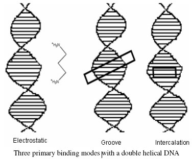
Oxidative DNA cleavage involves either oxidation of the deoxyribose moiety by abstraction of sugar hydrogen or oxidation of nulcleobases. It occurs in the presence of additives or photoinduced DNA cleavage agents.
Hydrolytic cleavage involves cleavage of phosphodiester bond to generate fragments which can be subsequently relegated. Hydrolytic cleavage mediated by nuclease enzymes which contain metal ions in their active site. Small metal complexes that promote the hydrolytic cleavage of DNA, therefore, are useful not only in molecular biology and drug desing but also in elucidating the precise role of metal ions in enzyme catalysis.
One of the most important approaches to drug development and current chemotherapy against some cancers and viral and parasitic diseases involve drugs which interact reversibly with DNA. Therefore, design of new metal complexes which can bind with specificity to DNA and bring about its cleavage are of importance in the development of new antitumor agents.