Coordinate System
A coordinate system allows one to place points on a plane in a precise way. In other words, each point in the plane is given a precise manner of specifying their location. The most useful coordinate system is called rectangular coordinates system (also known as Cartesian coordinate system), and Polar Coordinate system.
To define the atomic positions, numbers are needed - a set of coordinates. These may be external coordinates, referred to some set of coordinate axes, or they may be internal coordinates, defining the various interatomic distances and angles in the molecule of interest.
The geometry of a molecule can be described using one of three different methods.
The first is by using cartesian coordinates. Using the x-y-z coordinate system, the scientist must identify the coordinates for each atom in the molecule. However, this method is only efficient for small molecules.
The second method uses a molecular editor or graphical user interface (GUI). These are computer programs which allow you to construct various molecules. The program then automatically calculates the geometry of the molecule. GUIs work well for larger molecules.
The third method is called a Z-Matrix. The Z-Matrix is a simple, but rough, geometrical approximation. It works by identifying each atom in a molecule by a bond distance, bond angle and dihedral angle in relation to other atoms in the molecule. Z-Matrices work well for large molecules because the Z-Matrix can be easily converted to cartesian coordinates using Shodor's Z-Matrix Conversion Tool.
A dihedral angle is formed from four atoms, and helps to define the dimensionality of the molecule.
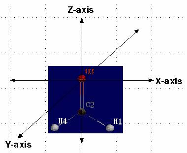
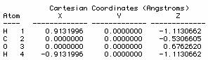
In chemistry, the Z-matrix is a way to represent a system built of atoms. A Z-matrix is also known as an internal coordinate representation. It provides a description of each atom in a molecule in terms of its atomic number, bond length, bond angle, and dihedral angle, the so-called internal coordinates, although it is not always the case that a Z-matrix will give information regarding bonding since the matrix itself is based on a series of vectors describing atomic orientations in space. However, it is convenient to write a Z-matrix in terms of bond lengths, angles, and dihedrals since this will preserve the actual bonding characteristics. The name arises because the Z-matrix assigns the second atom along the Z-axis from the first atom, which is at the origin.
Z-matrices can be converted to cartesian coordinates and back, as the information content is identical. They are used for creating input geometries for molecular systems in many molecular modelling and computational chemistry programs. A skillful choice of internal coordinates can make the interpretation of results straightforward. Also, since Z-matrices can contain molecular connectivity information (but do not always contain this information), quantum chemical calculations such as geometry optimization may be performed faster, because an educated guess is available for an initial Hessian matrix, and more natural internal coordinates are used rather than Cartesian coordinates. The Z-matrix representation is often preferred, because this allows symmetry to be enforced upon the molecule (or parts thereof) by setting certain angles as constant.
When constructing a Z-matrix, you should follow these steps:
Use this page to create a Z-matrix and convert it to Cartesian Coordinates for use in the ChemViz Program. This form permits you to convert a Z-matrix composed of 3 to 25 atoms. If you have more than 25 atoms, you should consider the use of a molecular editor. It can also be located at http://www.shodor.org/chemviz/babelex.html and http://www.shodor.org/chemviz/
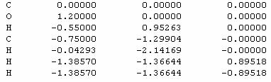
The methane molecule can be described by the following cartesian coordinates (in Ångströms):
C 0.000000 0.000000 0.000000
H 0.000000 0.000000 1.089000
H 1.026719 0.000000 -0.363000
H -0.513360 -0.889165 -0.363000
H -0.513360 0.889165 -0.363000
The corresponding Z-matrix, which starts from the carbon atom, could look like this:
C
H 1 1.089000
H 1 1.089000 2 109.4710
H 1 1.089000 2 109.4710 3 120.0000
H 1 1.089000 2 109.4710 3 -120.0000
Atom Name, Atom Connect, Bond Distance, Angle Connect, Bond Angle, Dihedral Connect, Dihedral Angle
Acetaldehyde:
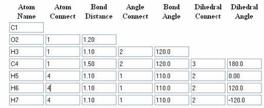
Building up of Acetaldehyde Molecule:
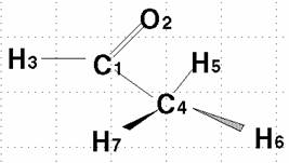
Here is the numbered molecule. Use this as a reference when following along in the example. Notice that the black arrow means that atom H7 is coming out of the screen and towards you. The shaded arrow H6 is going into the monitor.
These pictures show the five atoms that make up one plane. The included atoms are both carbons, the oxygen, and two hydrogens, each from opposite ends. This geometry is important when finding the dihedral angles.
|
C1 |
|
C1 |
|
|
|
O2 |
1 |
1.22 |
|
C1 |
|
|
|
|
|
O2 |
1 |
1.22 |
|
|
|
H3 |
1 |
1.09 |
2 |
120.0 |
|
C1 |
|
|
|
|
|
|
|
O2 |
1 |
1.22 |
|
|
|
|
|
H3 |
1 |
1.09 |
2 |
120.0 |
|
|
|
C4 |
1 |
1.54 |
2 |
120.0 |
3 |
180.0 |
|
C1 |
|
|
|
|
|
|
|
O2 |
1 |
1.22 |
|
|
|
|
|
H3 |
1 |
1.09 |
2 |
120.0 |
|
|
|
C4 |
1 |
1.54 |
2 |
120.0 |
3 |
180.0 |
|
H5 |
4 |
1.09 |
1 |
110.0 |
2 |
000.0 |
|
C1 |
|
|
|
|
|
|
|
O2 |
1 |
1.22 |
|
|
|
|
|
H3 |
1 |
1.09 |
2 |
120.0 |
|
|
|
C4 |
1 |
1.54 |
2 |
120.0 |
3 |
180.0 |
|
H5 |
4 |
1.09 |
1 |
110.0 |
2 |
000.0 |
|
H6 |
4 |
1.09 |
1 |
110.0 |
2 |
120.0 |
|
C1 |
|
|
|
|
|
|
|
O2 |
1 |
1.22 |
|
|
|
|
|
H3 |
1 |
1.09 |
2 |
120.0 |
|
|
|
C4 |
1 |
1.54 |
2 |
120.0 |
3 |
180.0 |
|
H5 |
4 |
1.09 |
1 |
110.0 |
2 |
000.0 |
|
H6 |
4 |
1.09 |
1 |
110.0 |
2 |
120.0 |
|
H7 |
4 |
1.09 |
1 |
110.0 |
2 |
-120.0 |
Cartesian coordinate system
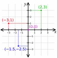
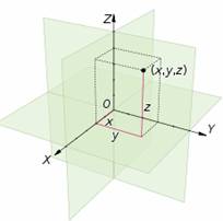
A Cartesian coordinate system specifies each point uniquely in a plane by a pair of numerical coordinates, which are the signed distances from the point to two fixed perpendicular directed lines, measured in the same unit of length.
Each reference line is called a coordinate axis or just axis of the system, and the point where they meet is its origin. The coordinates can also be defined as the positions of the perpendicular projections of the point onto the two axes, expressed as a signed distances from the origin.
Choosing a Cartesian coordinate system for a plane means choosing an ordered pair of lines (axes) at right angles to each other, a single unit of length for both axes, and an orientation for each axis. The point where the axes meet is taken as the origin for both axes, thus turning each axis into a number line. Each coordinate of a point p is obtained by drawing a line through p perpendicular to the associated axis, finding the point q where that line meets the axis, and interpreting q as a number of that number line.
Choosing a Cartesian coordinate system for a three-dimensional space means choosing an ordered triplet of lines (axes), any two of them being perpendicular; a single unit of length for all three axes; and an orientation for each axis. As in the two-dimensional case, each axis becomes a number line. The coordinates of a point p are obtained by drawing a line through p perpendicular to each axis, and reading the points where these lines meet the axes as three numbers of these number lines.
Alternatively, the coordinates of a point p can also be taken as the (signed) distances from p to the three planes defined by the three axes. If the axes are x, y, and z, then the x coordinate is the distance from the plane defined by the y and z axes. The distance is to be taken with the + or − sign, depending on which of the two half-spaces separated by that plane contains p. The y and z coordinates can be obtained in the same way from the (x,z) and (x,y) planes, respectively.
One can use the same principle to specify the position of any point in three-dimensional space by three Cartesian coordinates, its signed distances to three mutually perpendicular planes (or, equivalently, by its perpendicular projection onto three mutually perpendicular lines). In general, one can specify a point in space of any dimension n by use of n Cartesian coordinates, the signed distances from n mutually perpendicular hyperplanes.
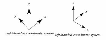
Once the x- and y-axes are specified, they determine the line along which the z-axis should lie, but there are two possible directions on this line. The two possible coordinate systems which result are called 'right-handed' and 'left-handed'. The standard orientation, where the xy-plane is horizontal and the z-axis points up (and the x- and the y-axis form a positively oriented two-dimensional coordinate system in the xy-plane if observed from above the xy-plane) is called right-handed or positive.
Cartesian coordinates are the foundation of analytic geometry, and provide enlightening geometric interpretations for many other branches of mathematics, such as linear algebra, complex analysis, differential geometry, multivariate calculus, group theory, and more. A familiar example is the concept of the graph of a function. Cartesian coordinates are also essential tools for most applied disciplines that deal with geometry, including astronomy, physics, engineering, and many more. They are the most common coordinate system used in computer graphics, computer-aided geometric design, and other geometry-related data processing.
Each axis may have different units of measurement associated with it (such as kilograms, seconds, pounds, etc.). Although four- and higher-dimensional spaces are difficult to visualize, the algebra of Cartesian coordinates can be extended relatively easily to four or more variables, so that certain calculations involving many variables can be done. (This sort of algebraic extension is what is used to define the geometry of higher-dimensional spaces.) Conversely, it is often helpful to use the geometry of Cartesian coordinates in two or three dimensions to visualize algebraic relationships between two or three of many non-spatial variables.
The graph of a function or relation is the set of all points satisfying that function or relation. For a function of one variable, f, the set of all points (x,y) where y = f(x) is the graph of the function f. For a function of two variables, g, the set of all points (x,y,z) where z = g(x,y) is the graph of the function g. A sketch of the graph of such a function or relation would consist of all the salient parts of the function or relation which would include its relative extrema, its concavity and points of inflection, any points of discontinuity and its end behavior. All of these terms are more fully defined in calculus. Such graphs are useful in calculus to understand the nature and behavior of a function or relation.
Polar Coordinates:
The usual Cartesian coordinate system can be quite difficult to use in certain situations. Some of the most common situations when Cartesian coordinates are difficult to employ involve those in which circular, cylindrical, or spherical symmetry is present. For these situations it is often more convenient to use a different coordinate system.
In mathematics, the polar coordinate system is a two-dimensional coordinate system in which each point on a plane is determined by a distance from a fixed point and an angle from a fixed direction.
The fixed point (analogous to the origin of a Cartesian system) is called the pole, and the ray from the pole with the fixed direction is the polar axis. The distance from the pole is called the radial coordinate or radius, and the angle is the angular coordinate, polar angle, or azimuth.
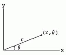
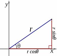
It is common to represent the point by an ordered pair (r,theta). Using standard trigonometry we can find conversions from Cartesian to polar coordinates
![]()
and from polar to Cartesian coordinates
![]()
There are two common methods for extending the polar coordinate system to three dimensions. In the cylindrical coordinate system, a z-coordinate with the same meaning as in Cartesian coordinates is added to the r and θ polar coordinates. Spherical coordinates take this a step further by converting the pair of cylindrical coordinates (r, z) to polar coordinates (ρ, φ) giving a triple (ρ, θ, φ).
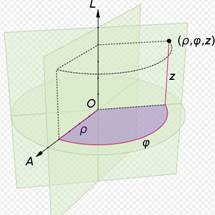
Cylindrical Polar Coordinate system:
A cylindrical coordinate system is a three-dimensional coordinate system, where each point is specified by the two polar coordinates of its perpendicular projection onto some fixed plane, and by its (signed) distance from that plane.
The polar coordinates may be called the radial distance or radius, and the angular position or azimuth, respectively. The third coordinate may be called the height or altitude (if the reference plane is considered horizontal), longitudinal position, or axial position. The line perpendicular to the reference plane that goes through its origin may be called the cylindrical axis or longitudinal axis.
Cylindrical coordinates are useful in connection with objects and phenomena that have some rotational symmetry about the longitudinal axis, such as water flow in a straight pipe with round cross-section, heat distribution in a metal cylinder, and so on.
The three coordinates (ρ, φ, z) of a point P are defined as:
Cylindrical coordinates are obtained by replacing the x and y coordinates with the polar coordinates r and theta (and leaving the z coordinate unchanged).
Thus, we have the following relations between Cartesian and cylindrical coordinates:
From cylindrical to Cartesian:
![]()
From Cartesian to cylindrical:
![]()
Coordinate range
– 0 ≤rc < ∞
0 ≤ θc ≤ 2π
– ∞ < z < ∞
Spherical Polar Coordinate system:
In mathematics, a spherical coordinate system is a coordinate system for three-dimensional space where the position of a point is specified by three numbers: the radial distance of that point from a fixed origin, its inclination angle measured from a fixed zenith direction, and the azimuth angle of its orthogonal projection on a reference plane that passes through the origin and is orthogonal to the zenith, measured from a fixed reference direction on that plane. The inclination angle is often replaced by the elevation angle measured from the reference plane.
The radial distance is also called the radius or radial coordinate, and the inclination may be called colatitude, zenith angle, normal angle, or polar angle.
In geography and astronomy, the elevation and azimuth (or quantities very close to them) are called the latitude and longitude, respectively; and the radial distance is usually replaced by an altitude (measured from a central point or from a sea level surface).
The concept of spherical coordinates can be extended to higher dimensional spaces and are then referred to as hyperspherical coordinates.
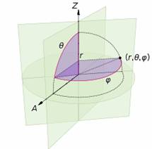
To define a spherical coordinate system, one must choose two orthogonal directions, the zenith and the azimuth reference, and an origin point in space. These choices determine a reference plane that contains the origin and is perpendicular to the zenith. The spherical coordinates of a point P are then defined as follows:
The sign of the azimuth is determined by choosing what is a positive sense of turning about the zenith. This choice is arbitrary, and is part of the coordinate system's definition.
The elevation angle is 90 degrees (π/2 radians) minus the inclination angle.
If the inclination is zero or 180 degrees (π radians), the azimuth is arbitrary. If the radius is zero, both azimuth and inclination are arbitrary.
In linear algebra, the vector from the origin O to the point P is often called the position vector of P.
The geographic coordinate system uses the azimuth and elevation of the spherical coordinate system to express locations on Earth, calling them respectively longitude and latitude. Just as the two-dimensional Cartesian coordinate system is useful on the plane, a two-dimensional spherical coordinate system is useful on the surface of a sphere. In this system, the sphere is taken as a unit sphere, so the radius is unity and can generally be ignored. This simplification can also be very useful when dealing with objects such as rotational matrices.
The spherical coordinate system is also commonly used in 3D game development to rotate the camera around the player's position.
The coordinates used in spherical coordinates are rho, theta, and phi. Rho is the distance from the origin to the point. Theta is the same as the angle used in polar coordinates. Phi is the angle between the z-axis and the line connecting the origin and the point.
The following are the relations between Cartesian and spherical coordinates:
From spherical to Cartesian:
![]()
From Cartesian to spherical:
![]()
Relations between cylindrical and spherical coordinates also exist:
From spherical to cylindrical:
![]()
From cylindrical to spherical:
Coordinate range:
0 ≤rs < ∞
0 ≤θs ≤ π
0 ≤φ ≤ 2π
MODELING SMALL MOLECULES
Small molecules can be modeled using co-ordinate system. Both Cartesian and polar co-ordinate systems were used to model the biomolecules. Especially the model of molecules depends upon the co-ordinates utilized in the co-ordinate system.
Model of a molecule can be visualized using molecular visualization tools. Example: Rasmol, Molmol, Swiss-PDB Viewer.
Rasmol: http://rasmol.org/
Molmol: http://hugin.ethz.ch/wuthrich/software/molmol/index.html
SPDBViewer: http://spdbv.vital-it.ch/
These visualization tools are free for academic purpose. One can download these softwares from their respective websites and can install in their computer. Molecules can be visualized through the installed programs.
These programs used to convert the co-ordinates in the structure file into the graphical display form. Different forms of display for example CPK model, ribbon model, wire model, stick model and Ball and stick model etc., are available. For all these display methods, the basic information was taken from the defined internal co-ordinates.
Usually structure files possess Cartesian co-ordinates. So these programs can simply help to view Cartesian co-ordinates in graphical form. Mostly PDB file format used for molecular structure. PDF format contains Cartesian co-ordinates x, y, z values which can be utilized for visualization purpose.
If the structure file present in other co-ordinate forms, for example, polar co-ordinate form, then these co-ordinate values first converted into cartesina co-ordinates and then be used for visualization purpose.
The methane molecule can be described by the following cartesian coordinates (in Ångströms):
C 0.000000 0.000000 0.000000
H 0.000000 0.000000 1.089000
H 1.026719 0.000000 -0.363000
H -0.513360 -0.889165 -0.363000
H -0.513360 0.889165 -0.363000
The corresponding Z-matrix, which starts from the carbon atom, could look like this:
C
H 1 1.089000
H 1 1.089000 2 109.4710
H 1 1.089000 2 109.4710 3 120.0000
H 1 1.089000 2 109.4710 3 -120.0000
Atom Name, Atom Connect, Bond Distance, Angle Connect, Bond Angle, Dihedral Connect, Dihedral Angle
MODELLING DNA
The structure of DNA is available in different conformations namely A, B, C and Z forms. The “B” form is the most common and biologically active form. In the “B” form DNA has some constant features namely the distance between residues is usually (tr) 3.4Ao; Number of residues per turn (pitch) is 10, the distance (length) is 34Ao, the angle tilt of the bases in DNA is 36o (tw). The bases are usually perpendicular to the helix axis (z-axis or dyad axis). The diameter of the helical structure is 20A. Two strands are antiparallel to each other.
For generation of standard DNA structures, with the helical symmetry, in addition to building blocks only two parameters are needed, viz. the base pair rise tr- which is the distance between the successive base pairs along the helical axis and the twist tw- which is the angle of rotation of the following base pair with respect to existing one, are needed. If one of the Cartesian axes (in general Z- axis) coincides with the helical axis of the molecule, we can generate the DNA polymer using set of rules given below.
Suppose xi, yi and zi are the coordinates of the ith atom in a building block, the coordinates of the same atom in the nth residue can be obtained by:
• Rotating coordinates of all the atoms in a block by angle (n-1).tw by a rotational transformation,
• Followed by translation of the unit along the helix axis by an amount (n-1).tr.
If the building blocks are in the Cylindrical polar coordinate system (ri, θiand zi designating coordinates of the ith atom ) the task is easier. In this case, radius rin of ith atom in the n th residue does not change with the residue number. Angle θin becomes θi + (n-1). tw, and Zin the z coordinates of the ith atom in the nth residue becomes Zin = zi + (n-1).tr. Thus Xin, Yin and Zin coordinates of ith atom of the nth residues are:
Generation of the opposite strand, can be done by using symmetry information in DNA. In the case of A and B forms of DNA, the dyad axis is along the X-axis. The projection of the sugar-phosphate backbone on the base plane has a mirror symmetry along this axis. As a result, the coordinates of the corresponding atom on the opposite strand (Xin', Yin', Zin' ) are given by:
where zi is the z coordinate of the same atom in the building block and Xin, Yin and Zin are the coordinates of the corresponding atom on the generating strand.
If the opposite strand is to be generated using cylindrical polar coordinates, the following relationship can be used:
These can be then converted to the Cartesian coordinates using following relation:
The advantage with the cylindrical polar coordinates is, that for the molecule with the cylindrical symmetry, the successive residues could be added by increasing Zi by tr rise per residue and θi by 360°/N where N is the number of residues per turn or axial symmetry.
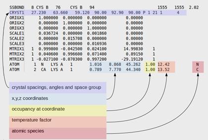
Here are a few lines from the PDB file for the DNA base pair structure directly above.
HEADER B-DNA
COMPND G-C B-DNA BASE PAIR
AUTHOR GENERATED BY GLACTONE
SEQRES 1 A 1 G
SEQRES 1 B 1 C
ATOM 1 P G A 1 -6.620 6.196 2.089
ATOM 2 OXT G A 1 -6.904 7.627 1.869
ATOM 3 O2P G A 1 -7.438 5.244 1.299
ATOM 4 O5' G A 1 -5.074 5.900 1.839
ATOM 5 C5' G A 1 -4.102 6.424 2.779
ATOM 6 C4' G A 1 -2.830 6.792 2.049
ATOM 7 O4' G A 1 -2.044 5.576 1.839
ATOM 8 C3' G A 1 -2.997 7.378 0.649
The last three columns are the XYZ coordinates of the atoms.
MODELLING PROTEINS
In contrast to DNA, proteins have wide range of structures due to the presence of different amino acid residues (20 basic amino acids). Due to the variation in monomeric residues , symmetric structures rarely occur in proteins. Protein models are represented by either Cartesian (both globular and fibrous proteins) or cylindrical (fibrous proteins) or spherical (globular proteins) co-ordinate system. Generally 3D structures of proteins were represented by using Cartesian co-ordinate system. The PDB file format is an example for Cartesian co-ordinate system (x, y, z).
When protein structure was represented by spherical co-ordinate system, three co-ordinates psi and phi angles and radius of the sphere were used for defining the structures. Especially secondary structures of polypeptide chains were usually represented by the psi and phi angles because variation in these angles leads to different secondary structures. Different secondary structures for different psi and phi angles were represented in the following table.
Gene Order:
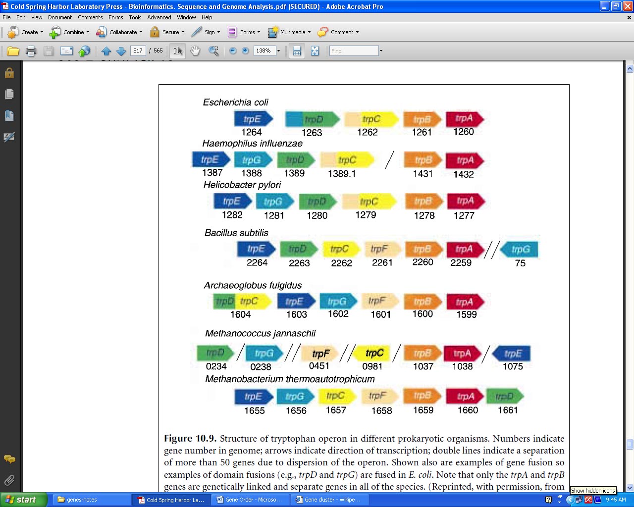
A Gene order is the permutation of genome arrangement. So far a fair amount of work trying to describe whether gene orders evolve according to a molecular clock (molecular clock hypothesis) or in jumps (punctuated equilibrium). Some researches on Gene orders of animals' mitochondrial gomone reveal that the mutation rate of gene orders is not a constant in some degrees. Two important observations have been made with regard to gene order: First, order is highly conserved in closely related species but becomes changed by rearrangements over evolutionary time. Second, group of genes that have a similar biological function tend to remain localized in a group or cluster.
In classical genetics, synteny describes the physical co-localization of genetic loci on the same chromosome within an individual or species. Synteny is a neologism meaning "on the same ribbon"; Greek: σύν, syn = along with + ταινία, tainiā = band.
The concept is related to genetic linkage: Linkage between two loci is established by the observation of lower-than-expected recombination frequencies between two or more loci. In contrast, any loci on the same chromosome are by definition syntenic, even if their recombination frequency cannot be distinguished from unlinked loci by practical experiments. Thus, in theory, all linked loci are syntenic, but not all syntenic loci are necessarily linked. Similarly, in genomics, the genetic loci on a chromosome are syntenic regardless of whether this relationship can be established by experimental methods such as DNA sequencing/assembly, genome walking, physical localization or hap-mapping.
Shared synteny describes preserved co-localization of genes on chromosomes of related species. During evolution, rearrangements to the genome such as chromosome translocations may separate two loci apart, resulting in the loss of synteny between them. Conversely, translocations can also join two previously separate pieces of chromosomes together, resulting in a gain of synteny between loci. Stronger-than-expected shared synteny can reflect selection for functional relationships between syntenic genes, such as combinations of alleles that are advantageous when inherited together, or shared regulatory mechanisms.
The analysis of synteny in the gene order sense has several applications in genomics. Shared synteny is one of the most reliable criteria for establishing the orthology of genomic regions in different species. Additionally, exceptional conservation of synteny can reflect important functional relationships between genes. For example, the order of genes in the "Hox cluster", which are key determinants of the animal body plan and which interact with each other in critical ways, is essentially preserved throughout the animal kingdom. Patterns of shared synteny or synteny breaks can also be used as characters to infer the phylogenetic relationships among several species, and even to infer the genome organization of extinct ancestral species. A qualitative distinction is sometimes drawn between macrosynteny, preservation of synteny in large portions of a chromosome, and microsynteny, preservation of synteny for only a few genes at a time.
Gene Cluster:
A gene cluster is a set of two or more genes that serve to encode for the same or similar products. Because populations from a common ancestor tend to possess the same varieties of gene clusters, they are useful for tracing back recent evolutionary history. Because of this, they were used by Luigi Luca Cavalli-Sforza to identify ethnic groups within Homo sapiens and their closeness to each other.
An example of a gene cluster is the Human β-globin gene cluster, which contains five functional genes and one non-functional gene for similar proteins. Hemoglobin molecules contain any two identical proteins from this gene cluster, depending on their specific role.
Gene clusters are created by the process of gene duplication and divergence. A gene is accidentally duplicated during cell division, so that its descendants have two copies of the gene, which initially code for the same protein or otherwise have the same function. In the course of subsequent evolution, they diverge, so that the products they code for have different but related functions, with the genes still being adjacent on the chromosome. This may happen repeatedly. The process was described by Susumu Ohno in his classic book Evolution by Gene Duplication (1970).
Gene Ontology: http://www.geneontology.org/
The Gene Ontology, or GO, is a major bioinformatics initiative to unify the representation of gene and gene product attributes across all species. The aims of the Gene Ontology project are threefold; firstly, to maintain and further develop its controlled vocabulary of gene and gene product attributes; secondly, to annotate genes and gene products, and assimilate and disseminate annotation data; and thirdly, to provide tools to facilitate access to all aspects of the data provided by the Gene Ontology project.
The Gene Ontology was originally constructed in 1998 by a consortium of researchers studying the genome of three model organisms: Drosophila melanogaster (fruit fly), Mus musculus (mouse), and Saccharomyces cerevisiae (brewers' or bakers' yeast). Many other model organism databases have joined the Gene Ontology consortium, contributing not only annotation data, but also contributing to the development of the ontologies and tools to view and apply the data. As of January 2008, GO contains over 24,500 terms applicable to a wide variety of biological organisms. There is a significant body of literature on the development and use of GO, and it has become a standard tool in the bioinformatics arsenal.
The Gene Ontology project provides ontology of defined terms representing gene product properties. The ontology covers three domains; cellular component, the parts of a cell or its extracellular environment; molecular function, the elemental activities of a gene product at the molecular level, such as binding or catalysis; and biological process, operations or sets of molecular events with a defined beginning and end, pertinent to the functioning of integrated living units: cells, tissues, organs, and organisms.
Each GO term within the ontology has a term name, which may be a word or string of words; a unique alphanumeric identifier; a definition with cited sources; and a namespace indicating the domain to which it belongs. Terms may also have synonyms, which are classed as being exactly equivalent to the term name, broader, narrower, or related; references to equivalent concepts in other databases; and comments on term meaning or usage. The GO ontology is structured as a directed acyclic graph, and each term has defined relationships to one or more other terms in the same domain, and sometimes to other domains. The GO vocabulary is designed to be species-neutral, and includes terms applicable to prokaryotes and eukaryotes, single and multicellular organisms.
id: GO:0000016
name: lactase activity
namespace: molecular_function
def: "Catalysis of the reaction: lactose + H2O = D-glucose + D-galactose." [EC:3.2.1.108]
synonym: "lactase-phlorizin hydrolase activity" BROAD [EC:3.2.1.108]
synonym: "lactose galactohydrolase activity" EXACT [EC:3.2.1.108]
xref: EC:3.2.1.108
xref: MetaCyc:LACTASE-RXN
xref: Reactome:20536
is_a: GO:0004553 ! hydrolase activity, hydrolyzing O-glycosyl compounds
Genome annotation is the practice of capturing data about a gene product, and GOES annotations use terms from the GO ontology to do so.
In addition to the gene product identifier and the relevant GO term, GO annotations have the following data:
The evidence code comes from the Evidence Code Ontology, a controlled vocabulary of codes covering both manual and automated annotation methods. For example, Traceable Author Statement (TAS) means a curator has read a published scientific paper and the metadata for that annotation bears a citation to that paper; Inferred from Sequence Similarity (ISS) means a human curator has reviewed the output from a sequence similarity search and verified that it is biologically meaningful. Annotations from automated processes (for example, remapping annotations created using another annotation vocabulary) are given the code Inferred from Electronic Annotation (IEA). As these annotations are not checked by a human, the GO Consortium considers them to be less reliable and does not include them in the data available online in AmiGO. Full annotation data sets can be downloaded from the GO website.
Gene product: Actin, alpha cardiac muscle 1, UniProtKB: P68032
GO term: heart contraction ; GO:0060047 (biological process)
Evidence code: Inferred from Mutant Phenotype (IMP)
Reference: PMID:17611253
Assigned by: UniProtKB, June 06, 2008
There are a large number of tools available both online and to download that use the data provided by the GO project. The vast majority of these come from third parties; the GO Consortium develops and supports two tools, AmiGO and OBO-Edit.
AmiGO is a web-based application that allows users to query, browse and visualize ontologies and gene product annotation data. In addition, it also has a BLAST tool, tools allowing analysis of larger data sets, and an interface to query the GO database directly.
AmiGO can be used online at the GO website to access the data provided by the GO Consortium, or can be downloaded and installed for local use on any database employing the GO database schema . It is free open source software and is available as part of the go-dev software distribution.
OBO-Edit is an open source, platform-independent ontology editor
developed and maintained by the Gene Ontology Consortium. It is implemented in
Java, and uses a graph-oriented approach to display and edit ontologies.
OBO-Edit includes a comprehensive search and filter interface, with the option
to render subsets of terms to make them visually distinct; the user interface
can also be customized according to user preferences. OBO-Edit also has a
reasoner that can infer links that have not been explicitly stated, based on
existing relationships and their properties. Although it was developed for
biomedical ontologies, OBO-Edit can be used to view, search and edit any
ontology. It is freely available to download.
Plasticity
The availability of the genome map has allowed investigation of issues such as the rates of recombination per physical distance and gene density across chromosomes. Phenotypic plasticity, in biology, describes the ability of an organism to change its phenotype in response to changes in the environment. Plasticity (tissues), in body tissues, plasticity refers to the ability of differentiated cells to undergo transdifferentiation.
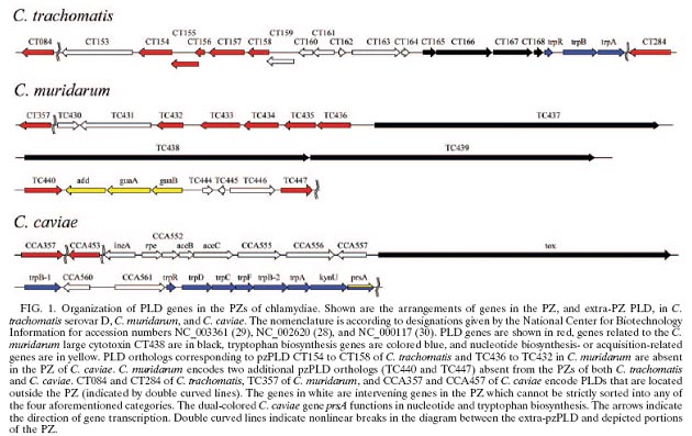
The genomes of different disease-causing C. trachomatis strains share more than 99% sequence identity. The genomes of different disease-causing C. trachomatis strains share more than 99% sequence identity. Genetic variations among these strains primarily map to a short region of their genomes termed the plasticity zone (PZ). Two strain-variable PZ gene families, the chlamydial cytotoxins and phospholipase D homologs, share homology with well-characterized virulence factors of other pathogens.
Most C. trachomatis genes are highly conserved, suggesting these "core component" genes perform critical functions. In contrast, variability in pathogenicity factors in the PZ among different C. trachomatis strains suggests these genes may be amenable to manipulation.
Members of the genus Chlamydia are obligate intracellular bacteria that are ubiquitous pathogens of mammals. Despite a broad range of host species, disease manifestations, and tissue tropisms of these organisms in nature, the genome sequences of chlamydiae are remarkably similar. Chlamydia trachomatis strains that cause distinct diseases in humans, including trachoma and chlamydial sexually transmitted diseases, as well as the more distantly related mouse pathogen Chlamydia muridarum, exhibit near genomic synteny. Comparative genomics suggests that genes necessary for the intracellular survival of chlamydiae are conserved, while genetic shift is limited to host- and tissue-specific virulence genes. Diversity in infection tropism and disease potential correlates with genes located in a hypervariable portion of the chlamydial genome termed the plasticity zone (PZ). Although previous studies have suggested virulence-related functions for many PZ genes, a large group of open reading frames encoding proteins with homology to the phospholipase D (PLD) family enzymes remain uncharacterized.
Gene Network
A gene regulatory network or genetic regulatory network (GRN) is a collection of DNA segments in a cell which interact with each other (indirectly through their RNA and protein expression products) and with other substances in the cell, thereby governing the rates at which genes in the network are transcribed into mRNA.
In general, each mRNA molecule goes on to make a specific protein (or set of proteins). In some cases this protein will be structural, and will accumulate at the cell-wall or within the cell to give it particular structural properties. In other cases the protein will be an enzyme; a micro-machine that catalyses a certain reaction, such as the breakdown of a food source or toxin. Some proteins though serve only to activate other genes, and these are the transcription factors that are the main players in regulatory networks or cascades. By binding to the promoter region at the start of other genes they turn them on, initiating the production of another protein, and so on. Some transcription factors are inhibitory.
In single-celled organisms regulatory networks respond to the external environment, optimising the cell at a given time for survival in this environment. Thus a yeast cell, finding itself in a sugar solution, will turn on genes to make enzymes that process the sugar to alcohol. This process, which we associate with wine-making, is how the yeast cell makes its living, gaining energy to multiply, which under normal circumstances would enhance its survival prospects.
In multicellular animals the same principle has been put in the service of gene cascades that control body-shape. Each time a cell divides, two cells result which, although they contain the same genome in full, can differ in which genes are turned on and making proteins. Sometimes a 'self-sustaining feedback loop' ensures that a cell maintains its identity and passes it on.
Boolean network
It provides output either in on or off state. One input and one output. The following example illustrates how a Boolean network can model a GRN together with its gene products (the outputs) and the substances from the environment that affect it (the inputs). Stuart Kauffman was amongst the first biologists to use the metaphor of Boolean networks to model genetic regulatory networks.
The validity of the model can be tested by comparing simulation results with time series observations.
Continuous networks
Many components act as input and output of one event act as input of an another input. Example: Cellular differentiation and morphogenesis.
Continuous network models of GRNs are an extension of the boolean networks described above. Nodes still represent genes and connections between them regulatory influences on gene expression. Genes in biological systems display a continuous range of activity levels and it has been argued that using a continuous representation captures several properties of gene regulatory networks not present in the Boolean model. Formally most of these approaches are similar to an artificial neural network, as inputs to a node are summed up and the result serves as input to a sigmoid function, but proteins do often control gene expression in a synergistic, i.e. non-linear, way. However there is now a continuous network model that allows grouping of inputs to a node thus realizing another level of regulation. This model is formally closer to a higher order recurrent neural network. The same model has also been used to mimic the evolution of cellular differentiation and even multicellular morphogenesis.
Stochastic gene networks
It represents stepwise events. Example: transcription, translation
Recent experimental results have demonstrated that gene expression is a stochastic process. Thus, many authors are now using the stochastic formalism, after the work by. Works on single gene expression and small synthetic genetic networks, such as the genetic toggle switch of Tim Gardner and Jim Collins, provided additional experimental data on the phenotypic variability and the stochastic nature of gene expression. The first versions of stochastic models of gene expression involved only instantaneous reactions and were driven by the Gillespie algorithm.
Operon concept is an example to explain gene network.
Gene Density
Gene density refers to the occurrence of more genes in a defined area of genome. It is measured with the help physical map. Gene density, as measured by the number of cDNAs hybridizing to YACs within physical map intervals, varies by a factor of more than two between chromosome clusters and their arms, again with a relatively sharp boundary. The availability of the genome map has allowed investigation of issues such as the rates of recombination per physical distance and gene density across chromosomes.
SEGMENT DUPLICATIONS
Segmental duplications are segments of DNA with near-identical sequence. Segmental duplications (SDs or LCRs) have had roles in creating new primate genes reflected on human genetic variation. In human genome chromosomes Y and 22 have the greatest SDs proportion: 50.4% and 11.9%.
Low copy repeats (also low-copy repeats or LCRs) are highly homologous sequence elements within the eukaryotic genome arising from segmental duplication. They are typically 10–300 kb in length, and bear >95% sequence identity. Though rare in most mammals, LCRs comprise a large portion of the human genome due to a significant expansion during primate evolution. Misalignment of LCRs during non-allelic homologous recombination (NAHR) is an important mechanism underlying the chromosomal microdeletion disorders as well as their reciprocal duplication partners. Many LCRs are concentrated in "hotspots", such as the 17p11-12 region, 27% of which is composed of LCR sequence.
Segments of DNA with near-identical sequence (segmental duplications or duplicons) in the human genome can be hot spots or predisposition sites for the occurrence of non-allelic homologous recombination or unequal crossing-over leading to genomic mutations such as deletion, duplication, inversion or translocation. These structural alterations, in turn, can cause dosage imbalance of genetic material or lead to the generation of new gene products resulting in diseases defined as genomic disorders.
On the basis of the June 2002 (NCBI Build 30) human genome assembly, a total of 107.4 Mb (3.53%) of the human genome content (3,043.1 Mb) were found to be involved in recent segmental duplications by BLAST analysis criteria. This content is composed of more than 1,530 distinct intrachromosomal segmental duplications (80.3 Mb or 2.64% of the total genome) and 1,637 distinct interchromosomal duplications (43.8 Mb or 1.44% of the total genome). In addition, 29% of all duplications are located in unfinished regions of the current genome assembly. Our results are shown using the Generic Genome Browser. We have also found that 38% of the duplications (52.3 Mb) can be considered as tandem duplications - defined here as two related duplicons separated by less than 200 kb.
The size, orientation, and contents of segmental duplications are highly variable and most of them show great organizational complexity. This is perhaps due to successive transposition and rearrangement events leading to the creation of segmental duplications. In many cases, a contiguous duplicon is organized into multiple modules with different orientations and sizes. The characterization of most large segmental duplications is complicated by the fact that many of them (29% of all duplications) are only represented as draft sequences from the current genome assembly.
The segmental duplication map of the human genome should serve as a guide for investigation of the role of duplications in genomic disorders, as well as their contributions to normal human genomic variability.
BLAST and detection of segmental duplication
Each BLAST report was sorted by chromosomal coordinates. All identical hits (same coordinate alignments), including suboptimal BLAST alignments recognized by multiple, overlapping alignments, as well as mirror hits (reverse coordinate alignments) from the BLAST results of the intrachromosomal set were removed. Contiguous alignments separated by a distance of less than 3 kb, then 5 kb, and subsequently 9 kb were joined (stepwise) into modules in order to traverse masked repetitive sequences and to overcome breaks in the BLAST alignments caused by insertions/deletions and sequence gaps. Such contiguous sequence alignment modules represent sequence similarity between the subject and query chromosome sequence in question (at their respective positional coordinates). This pairwise sequence comparison procedure serves as a rapid and robust way to detect duplication relationships. However, because of the use of masked sequences, our method would only yield a poor (on average 0.1-0.5 kb) resolution for the determination of the precise duplication alignment boundaries. Results were classified as either duplications or 'questionable' results based on sequencing status of the region and the percent sequence similarity between the detected alignments. Questionable duplications are results that fall within regions containing draft sequences with > 99.5 % detected sequence identity with another region.
TANDEM REPEATS
Tandem repeats occur in DNA when a pattern of two or more nucleotides is repeated and the repetitions are directly adjacent to each other. An example would be: A-T-T-C-G-A-T-T-C-G-A-T-T-C-G in which the sequence A-T-T-C-G is repeated three times. They include three subclasses: satellites, minisatellites and microsatellites.
Satellites
The size of a satellite DNA ranges from 100 kb to over 1 Mb. In humans, a well known example is the alphoid DNA located at the centromere of all chromosomes. Its repeat unit is 171 bp and the repetitive region accounts for 3-5% of the DNA in each chromosome. Other satellites have a shorter repeat unit. Most satellites in humans or in other organisms are located at the centromere.
Minisatellites
The size of a minisatellite ranges from 1 kb to 20 kb. One type of minisatellites is called variable number of tandem repeats (VNTR). Its repeat unit ranges from 9 bp to 80 bp. They are located in non-coding regions. The number of repeats for a given minisatellite may differ between individuals. This feature is the basis of DNA fingerprinting. Another type of minisatellites is the telomere. In a human germ cell, the size of a telomere is about 15 kb. In an aging somatic cell, the telomere is shorter. The telomere contains tandemly repeated sequence GGGTTA.
Microsatellites are also known as short tandem repeats (STR), because a repeat unit consists of only 1 to 6 bp and the whole repetitive region spans less than 150 bp. Similar to minisatellites, the number of repeats for a given microsatellite may differ between individuals. Therefore, microsatellites can also be used for DNA fingerprinting. In addition, both microsatellite and minisatellite patterns can provide information about paternity.
Uses:
Tandem repeat describes a pattern that helps determine an individual's inherited traits.
Tandem repeats can be very useful in determining parentage. Short tandem repeats are used for certain genealogical DNA tests.
DNA is examined from microsatellites within the chromosomal DNA. Minisatellite is another way of saying special regions of the loci. Polymerase chain reaction (or PCR) is performed on the minisatellite areas. The PCR must be performed on each organism being tested. The amplified material is then run through electrophoresis. By checking the percentage of bands that match, parentage is determined.
In the field of Computer Science, tandem repeats in strings (e.g., DNA sequences) can be efficiently detected using suffix trees or suffix arrays.
Studies in 2004 linked the unusual genetic plasticity of dogs to mutations in tandem repeats.
TRANSPOSABLE ELEMENTS
Transposable elements -- also known as transposons or "jumping genes" -- are genes that can move themselves or a copy of themselves from one chromosome to another. Because they can move to different chromosomes, they contribute to the creation of new genes.
Transposable elements (TEs), also known as "jumping genes," are DNA sequences that move from one location on the genome to another. These elements were first identified more than 50 years ago by geneticist Barbara McClintock of Cold Spring Harbor Laboratory in New York. Biologists were initially skeptical of McClintock's discovery. Over the next several decades, however, it became apparent that not only do TEs "jump," but they are also found in almost all organisms (both prokaryotes and eukaryotes) and typically in large numbers. For example, TEs make up approximately 50% of the human genome and up to 90% of the maize genome.
Today, scientists know that there are many different types of TEs, as well as a number of ways to categorize them. One of the more common divisions is between those TEs that require reverse transcription (i.e., the transcription of RNA into DNA) in order to transpose and those that do not. The former elements are known as retrotransposons or class 1 TEs, whereas the latter are known as DNA transposons or class 2 TEs. The Ac/Ds system that McClintock discovered falls in the latter category.
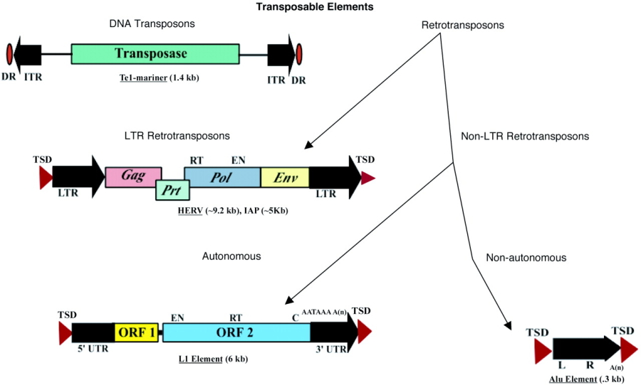
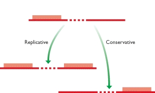
All complete or "autonomous" class 2 TEs encode the protein transposase, which they require for insertion and excision. Some of these TEs also encode other proteins. Note that DNA transposons never use RNA intermediaries—they always move on their own, inserting or excising themselves from the genome by means of a so-called "cut and paste" mechanism.
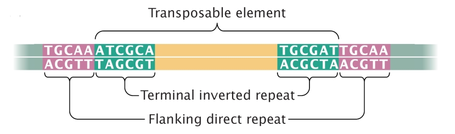
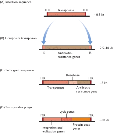
Class 2 TEs are characterized by the presence of terminal inverted repeats, about 9 to 40 base pairs long, on both of their ends. As the name suggests and as Figure 3 shows, terminal inverted repeats are inverted complements of each other; for instance, the complement of ACGCTA (the inverted repeat on the right side of the TE in the figure) is TGCGAT (which is the reverse order of the terminal inverted repeat on the left side of the TE in the figure). One of the roles of terminal inverted repeats is to be recognized by transposase.
In addition, all TEs in both class 1 and class 2 contain flanking direct repeats (Figure 3). Flanking direct repeats are not actually part of the transposable element; rather, they play a role in insertion of the TE. Moreover, after a TE is excised, these repeats are left behind as "footprints." Sometimes, these footprints alter gene expression (i.e., expression of the gene in which they have been left behind) even after their related TE has moved to another location on the genome.
Less than 2% of the human genome is composed of class 2 TEs. This means that the majority of the substantial portion of the human genome that is mobile consists of the other major class of TEs—the retrotransposons.
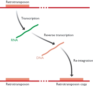
Unlike class 2 elements, class 1 elements—also known as retrotransposons—move through the action of RNA intermediaries. In other words, class 1 TEs do not encode transposase; rather, they produce RNA transcripts and then rely upon reverse transcriptase enzymes to reverse transcribe the RNA sequences back into DNA, which is then inserted into the target site.
Both class 1 and class 2 TEs can be either autonomous or nonautonomous. Autonomous TEs can move on their own, while nonautonomous elements require the presence of other TEs in order to move. This is because nonautonomous elements lack the gene for the transposase or reverse transcriptase that is needed for their transposition, so they must "borrow" these proteins from another element in order to move. Ac elements, for example, are autonomous because they can move on their own, whereas Ds elements are nonautonomous because they require the presence of Ac in order to transpose.
Applications
The first TE was discovered in the plant maize (Zea mays, corn species), and is named dissociator (Ds). Likewise, the first TE to be molecularly isolated was from a plant (Snapdragon). Appropriately, TEs have been an especially useful tool in plant molecular biology. Researchers use them as a means of mutagenesis. In this context, a TE jumps into a gene and produces a mutation. The presence of such a TE provides a straightforward means of identifying the mutant allele, relative to chemical mutagenesis methods.
Sometimes the insertion of a TE into a gene can disrupt that gene's function in a reversible manner, in a process called insertional mutagenesis; transposase-mediated excision of the DNA transposon restores gene function. This produces plants in which neighboring cells have different genotypes. This feature allows researchers to distinguish between genes that must be present inside of a cell in order to function (cell-autonomous) and genes that produce observable effects in cells other than those where the gene is expressed.
TEs are also a widely used tool for mutagenesis of most experimentally tractable organisms. The Sleeping Beauty transposon system has been used extensively as an insertional tag for identifying cancer genes
The Tc1/mariner-class of TEs Sleeping Beauty transposon system, awarded as the Molecule of the Year 2009 is active in mammalian cells and are being investigated for use in human gene therapy.
PSEUDOGENES
Pseudogenes are dysfunctional relatives of known genes that have lost their protein-coding ability or are otherwise no longer expressed in the cell. Although some do not have introns or promoters (these pseudogenes are copied from mRNA and incorporated into the chromosome and are called processed pseudogenes), most have some gene-like features (such as promoters, CpG islands, and splice sites), they are nonetheless considered nonfunctional, due to their lack of protein-coding ability resulting from various genetic disablements (stop codons, frameshifts, or a lack of transcription) or their inability to encode RNA (such as with rRNA pseudogenes). Thus the term, coined in 1977 by Jacq, et al., is composed of the prefix pseudo, which means false, and the root gene, which is the central unit of molecular genetics.
Because pseudogenes are generally thought of as the last stop for genomic material that is to be removed from the genome, they are often labeled as junk DNA. Nonetheless, pseudogenes contain fascinating biological and evolutionary histories within their sequences. This is due to a pseudogene's shared ancestry with a functional gene: in the same way that Darwin thought of two species as possibly having a shared common ancestry followed by millions of years of evolutionary divergence, a pseudogene and its associated functional gene also share a common ancestor and have diverged as separate genetic entities over millions of years.
Properties of pseudogenes
Pseudogenes are characterized by a combination of homology to a known gene and nonfunctionality. That is, although every pseudogene has a DNA sequence that is similar to some functional gene, they are nonetheless unable to produce functional final products (nonfunctionality). Pseudogenes are quite difficult to identify and characterize in genomes, because the two requirements of homology and nonfunctionality are implied through sequence calculations and alignments rather than biologically proven.
Types of pseudogenes
There are three main types of pseudogenes, all with distinct mechanisms of origin and characteristic features. The classifications of pseudogenes are as follows:
Pseudogenes can complicate molecular genetic studies. For example, a researcher who wants to amplify a gene by PCR may simultaneously amplify a pseudogene that shares similar sequences. This is known as PCR bias or amplification bias. Similarly, pseudogenes are sometimes annotated as genes in genome sequences. Processed pseudogenes often pose a problem for gene prediction programs, often being misidentified as real genes or exons. It has been proposed that identification of processed pseudogenes can help improve the accuracy of gene prediction methods. It has also been shown that the parent sequences that give rise to processed pseudogenes lose their coding potential faster than those giving rise to non-processed pseudogenes.
Noncoding conservation
Whole genome comparisons between species that are either closely related or more phylogenetically separated—such as human, mouse, and dog—have revealed a subset of sequences that neither code for proteins nor are transcribed, yet are nevertheless conserved, but whose function is as yet unknown (conserved nongenic sequences, or CNGs). Emmanouil Dermitzakis and colleagues at the University of Geneva employed data-mining techniques to examine the extent to which these CNGs are spread across 14 mammalian species. In the October 2 Science, they report that CNGs are highly conserved in 14 species and constitute a new class of sequences that are even more evolutionarily constrained than protein coding regions (Science, DOI:10.1126/science.1087047, October 2, 2003).
In addition to protein coding sequence, the human genome contains a significant amount of regulatory DNA, the identification of which is proving somewhat recalcitrant to both in silico^ and functional methods. An approach that has been used with some success is comparative sequence analysis, whereby equivalent genomic regions from different organisms are compared in order to identify both similarities and differences. In general, similarities in sequence between highly divergent organisms imply functional constraint. We have used a whole-genome comparison between humans and the pufferfish, Fugu rubripes, to identify nearly 1,400 highly conserved non-coding sequences. Given the evolutionary divergence between these species, it is likely that these sequences are found in, and furthermore are essential to, all vertebrates. Most, and possibly all, of these sequences are located in and around genes that act as developmental regulators. Some of these sequences are over 90% identical across more than 500 bases, being more highly conserved than coding sequence between these two species. Despite this, we cannot find any similar sequences in invertebrate genomes. In order to begin to functionally test this set of sequences, we have used a rapid in vivo assay system using zebrafish embryos that allows tissue-specific enhancer activity to be identified. Functional data is presented for highly conserved non-coding sequences associated with four unrelated developmental regulators (SOX21, PAX6, HLXB9, and SHH), in order to demonstrate the suitability of this screen to a wide range of genes and expression patterns. Of 25 sequence elements tested around these four genes, 23 show significant enhancer activity in one or more tissues. We have identified a set of non-coding sequences that are highly conserved throughout vertebrates. They are found in clusters across the human genome, principally around genes that are implicated in the regulation of development, including many transcription factors. These highly conserved non-coding sequences are likely to form part of the genomic circuitry that uniquely defines vertebrate development.
Identification and characterisation of cis-regulatory regions within the non-coding DNA of vertebrate genomes remain a challenge for the post-genomic era. The idea that animal development is controlled by cis-regulatory DNA elements (such as enhancers and silencers) is well established and has been elegantly described in invertebrates such as Drosophila and the sea urchin. These elements are thought to comprise clustered target sites for large numbers of transcription factors and collectively form the genomic instructions for developmental gene regulatory networks (GRNs). However, relatively little is known about GRNs in vertebrates. Any approach to elucidate such networks necessitates the discovery of all constituent cis-regulatory elements and their genomic locations. Unfortunately, initial in silico identification of such sequences is difficult, as current knowledge of their syntax or grammar is limited. By contrast, computational approaches for protein-coding exon prediction are well established, based on their characteristic sequence features, evolutionary conservation across distant species, and the availability of cDNAs and expressed sequence tags (ESTs), which greatly facilitate their annotation.
The completion of a number of vertebrate genome sequences, as well as the concurrent development of genomic alignment, visualisation, and analytical bioinformatics tools, has made large genomic comparisons not only possible but an increasingly popular approach for the discovery of putative cis-regulatory elements. Comparing DNA sequences from different organisms provides a means of identifying common signatures that may have functional significance. Alignment algorithms optimise these comparisons so that slowly evolving regions can be anchored together and highlighted against a background of more rapidly evolving DNA that is free of any functional constraints.
Another highly successful approach to increasing the resolving power of comparative analyses is to use multi-species alignments combining both closely related and highly divergent organisms. By using large evolutionary distances, even the slowest-evolving neutral DNA has reached equilibrium, thereby significantly improving the signal to noise ratio in genomic alignments. Although non-coding sequences generally lack sequence conservation between highly divergent species, there are a number of striking examples where comparison between human and pufferfish (Fugu rubripes) gene regions has readily identified highly conserved non-coding sequences that have been shown to have some function in vivo. Humans and Fugu last shared a common ancestor around 450 million years ago, predating the emergence of the majority of all extant vertebrates, implying that any non-coding sequences conserved between these two species are likely to be fundamental to vertebrate life. The Fugu genome has the added advantage of being highly compact, reducing intronic and intergenic distances almost 10-fold. Without exception, all reported examples of non-coding conservation between these two species have been associated with genes that play critical roles in development. This suggests that some aspects of developmental regulation are common to all vertebrates and that whole-genome comparisons may be particularly powerful in identifying regulatory networks of this kind.
SUFFIX TREE
Molecular Biologists often search for sequence patterns in molecular genetic data. Consider for example the text t= ACCGTC and the pattern P= C. A string search should tell us as efficiently as possible that occurs in at positions 2, 3, and 6. Classical results in computer science have lead to algorithms that achieve this in time proportional to the length of T.
Suffix trees are an ideal data structure for improving on this result in cases where the text is stable and needs to be searched repeatedly. Suffix trees are an index structure of the text, which can be built in linear time [249]. Once built, the text can be searched for a pattern in time proportional to the length of the pattern rather than in time proportional to the length of the text.
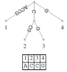
A suffix tree (t) is a special kind of tree associated with a string S, where |s| = n. has as many leaves as the string has characters and these leaves are labeled 1,….n. Each edge in the tree is labeled with a substring of S. The defining feature of the suffix tree is that by concatenating the strings from the root along the edges leading to leaf i, the suffix S[i…n] is obtained. Figure shows a suffix tree for S= ACCG. If you start reading at its root and follow the path leading to leaf 2, you obtain the string CCG. This is the suffix that starts at position 2 in S.
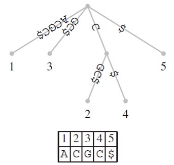
Notice that it is possible that a suffix is a prefix of another suffix. For example, in S=ACGC the suffix S[4..4]=C is a prefix of the suffix S[2..4]=CGC. In this case, no suffix tree corresponding to S exists, as the path labeled S [4..4] would not end at a leaf. A simple method for guaranteeing the existence of a suffix tree is to ensure that the last letter of S does not occur anywhere else in S. In practice, a sentinel or terminator symbol, often denoted as $ is added to S and T is constructed from S$.
Suffix Tree Construction
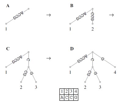
Suffix trees are usually constructed through a series of intermediate trees. One possible naıve algorithm proceeds as follows: Construct a root and a leaf node labeled 1 . The edge connecting these two nodes is labeled S[1..n]. This initial tree is converted to the final structure by successively fitting the suffices, S[1..n], 1<i<n, into the intermediate trees. As demonstrated in Figure, each of these fitting steps proceeds by matching the suffix along the edge labels starting at the root until a mismatch is encountered. Remember that due to the sentinel character a mismatch is guaranteed to occur. Once this is found, there are two possibilities:
1. The match ends at the last letter of an edge label leading to node v. In this case, an edge labeled with the mismatched part of the suffix is attached to v. This edge leads to a leaf labeled with the start position of the current suffix. Examples of this are steps Aà B and Cà D in Figure.
2. The match ends inside an edge label. In this case, an interior node v is inserted just behind the end of the match. In addition, a leaf labeled i is attached to v via an edge labeled with the mismatched part of the suffix. An example of this splitting of an edge is step Bà C in Figure.
generalized suffix tree
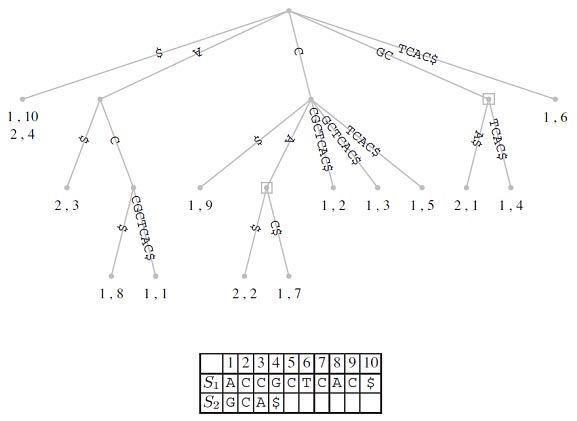
So far, we have constructed suffix trees just from a single string. However, it is straight forward to generate what is known as a generalized suffix tree representing more than one string. Consider the two strings S1 and S2. We can proceed by first constructing the suffix tree for S1 and then inserting into this every suffix of S2. All we need to do is change the leaf labels such that they now consist of pairs of numbers identifying both the string of origin and the position within that string. As an example, consider S1=ACCGCTCAC; the corresponding suffix tree is shown in Figure. If we insert into this suffix tree S2=GCA, we obtain the tree topology shown in Figure. Using the new labeling scheme for leaves, generalized suffix trees of an arbitrary number of strings can be constructed. This opens the way for solving the longest common substring problem.
This has important biological applications where unique and repeat sequences play a central role in many fundamental as well as biotechnological problems. Finally, suffix trees can also be used for rapid inexact string matching, where <=k, mismatches between P and its occurrence in T are allowed.
Genome Anatomy
Genome anatomy is the structure of all the genetic information in the haploid portion of chromosomes of a cell. Biologists recognize that the living world comprises two types of organism:
1. Eukaryotes, whose cells contain membrane-bound compartments, including a nucleus and organelles such as mitochondria and, in the case of plant cells, chloroplasts. Eukaryotes include animals, plants, fungi and protozoa.
2. Prokaryotes whose cells were lack extensive internal compartments. There are two very different groups of prokaryotes, distinguished from one another by characteristic genetic and biochemical features:
a. the bacteria, which include most of the commonly encountered prokaryotes such as the gram-negatives (e.g. E. coli), the gram-positives (e.g. Bacillus subtilis), the cyanobacteria (e.g. Anabaena) and many more;
b. the archaea, which are less well-studied, and have mostly been found in extreme environments such as hot springs, brine pools and anaerobic lake bottoms.
Genome anatomy comparison
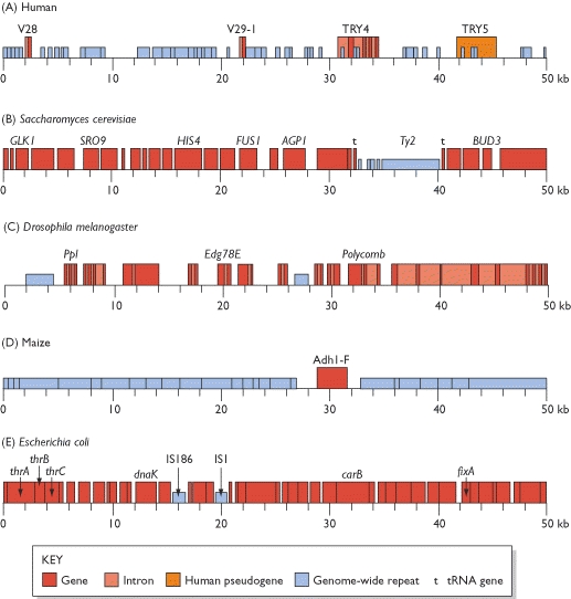
The picture that emerges is that the genetic organization of the yeast genome is much more economical than that of the human version. The genes themselves are more compact, having fewer introns, and the spaces between the genes are relatively short, with much less space taken up by genome-wide repeats and other non-coding sequences. The hypothesis that more complex organisms have less compact genomes holds when other species are examined. If we agree that a fruit fly is more complex than a yeast cell but less complex than a human then we would expect the organization of the fruit-fly genome to be intermediate between that of yeast and humans. The 50-kb segment of the fruit-fly genome having 11 genes, that is more than in the human segment but fewer than in the yeast sequence. All of these genes are discontinuous, but seven have just one intron each. The gene density in the fruit-fly genome is intermediate between that of yeast and humans, and the average fruit-fly gene has many more introns than the average yeast gene but still three times fewer than the average human gene.
The comparison between the yeast, fruit-fly and human genomes also holds true when we consider the genome-wide repeats. These make up 3.4% of the yeast genome, about 12% of the fruit-fly genome, and 44% of the human genome. It is beginning to become clear that the genome-wide repeats play an intriguing role in dictating the compactness or otherwise of a genome. This is strikingly illustrated by the maize genome, which at 5000 Mb is larger than the human genome but still relatively small for a flowering plant. Only a few limited regions of the maize genome have been sequenced, but some remarkable results have been obtained, revealing a genome dominated by repetitive elements. The figure shows a 50-kb segment of this genome, either side of one member of a family of genes coding for the alcohol dehydrogenase enzymes. This is the only gene in this 50-kb region, although there is a second one, of unknown function, approximately 100 kb beyond the right-hand end of the sequence shown here. Instead of genes, the dominant feature of this genome segment is the genome-wide repeats. The majority of these are of the LTR element type, which comprise virtually all of the non-coding part of the segment, and on their own are estimated to make up approximately 50% of the maize genome. It is becoming clear that one or more families of genome-wide repeats have undergone a massive proliferation in the genomes of certain species.
The c-value paradox is the non-equivalence between genome size and gene number that is seen when comparisons are made between some eukaryotes. A good example is provided by Amoeba dubia which, being a protozoan, might be expected to have a genome of 100–500 kb, similar to other protozoa such as Tetrahymena pyriformis. In fact the Amoeba genome is over 200 000 Mb. Similarly, we might guess that the genomes of crickets are similar in size to those of other insects, but these bugs have genomes of approximately 2000 Mb, 11 times that of the fruit fly.
Eukaryotes genomes:
Humans are fairly typical eukaryotes and the human genome is in many respects a good model for eukaryotic genomes in general. All of the eukaryotic nuclear genomes that have been studied are, like the human version, divided into two or more linear DNA molecules, each contained in a different chromosome; all eukaryotes also possess smaller, usually circular, mitochondrial genomes. The only general eukaryotic feature not illustrated by the human genome is the presence in plants and other photosynthetic organisms of a third genome, located in the chloroplasts.
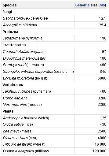
Although the basic physical structures of all eukaryotic nuclear genomes are similar, one important feature is very different in different organisms. This is genome size, the smallest eukaryotic genomes being less than 10 Mb in length, and the largest over 100 000 Mb. As can be seen in table, this size range coincides to a certain extent with the complexity of the organism, the simplest eukaryotes such as fungi having the smallest genomes, and higher eukaryotes such as vertebrates and flowering plants having the largest ones. This might appear to make sense as one would expect the complexity of an organism to be related to the number of genes in its genome - higher eukaryotes need larger genomes to accommodate the extra genes. However, the correlation is far from precise: if it was, then the nuclear genome of the yeast S. cerevisiae, which at 12 Mb is 0.004 times the size of the human nuclear genome, would be expected to contain 0.004 × 35 000 genes, which is just 140. In fact the S. cerevisiae genome contains about 5800 genes.
The yeast genome segment, which comes from chromosome III (the first eukaryotic chromosome to be sequenced), has the following distinctive features:
· It contains more genes than the human segment. This region of yeast chromosome III contains 26 genes thought to code for proteins and two that code for transfer RNAs (tRNAs), short non-coding RNA molecules involved in reading the genetic code during protein synthesis.
· Relatively few of the yeast genes are discontinuous. In this segment of chromosome III none of the genes are discontinuous. In the entire yeast genome there are only 239 introns, compared with over 300 000 in the human genome.
· There are fewer genome-wide repeats. This part of chromosome III contains a single long terminal repeat (LTR) element, called Ty2, and four truncated LTR elements called delta sequences. These five genome-wide repeats make up 13.5% of the 50-kb segment, but this figure is not entirely typical of the yeast genome as a whole. When all 16 yeast chromosomes are considered, the total amount of sequence taken up by genome-wide repeats is only 3.4% of the total. In humans, the genome-wide repeats make up 44% of the genome.
Prokaryotic genomes
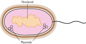
Prokaryotic genomes are very different from eukaryotic ones. There is some overlap in size between the largest prokaryotic and smallest eukaryotic genomes, but on the whole prokaryotic genomes are much smaller. For example, the E. coli K12 genome is just 4639 kb, two-fifths the size of the yeast genome, and has only 4405 genes. The physical organization of the genome is also different in eukaryotes and prokaryotes. The traditional view has been that an entire prokaryotic genome is contained in a single circular DNA molecule. As well as this single ‘chromosome’, prokaryotes may also have additional genes on independent smaller, circular or linear DNA molecules called plasmids. Genes carried by plasmids are useful, coding for properties such as antibiotic resistance or the ability to utilize complex compounds such as toluene as a carbon source, but plasmids appear to be dispensable - a prokaryote can exist quite effectively without them. We now know that this traditional view of the prokaryotic genome has been biased by the extensive research on E. coli, which has been accompanied by the mistaken assumption that E. coli is a typical prokaryote. In fact, prokaryotes display a considerable diversity in genome organization, some having a unipartite genome, like E. coli, but others being more complex. Borrelia burgdorferi B31, for example, has a linear chromosome of 911 kb, carrying 853 genes, accompanied by 17 or 18 linear and circular molecules, which together contribute another 533 kb and at least 430 genes. Multipartite genomes are now known in many other bacteria and archaea.
In one respect, E. coli is fairly typical of other prokaryotes. After our discussion of eukaryotic gene organization, it will probably come as no surprise to learn that prokaryotic genomes are even more compact than those of yeast and other lower eukaryotes. It is immediately obvious that there are more genes and less space between them, with 43 genes taking up 85.9% of the segment. Some genes have virtually no space between them: thrA and thrB, for example, are separated by a single nucleotide, and thrC begins at the nucleotide immediately following the last nucleotide of thrB. These three genes are an example of an operon, a group of genes involved in a single biochemical pathway (in this case, synthesis of the amino acid threonine) and expressed in conjunction with one another. Operons have been used as model systems for understanding how gene expression is regulated. In general, prokaryotic genes are shorter than their eukaryotic counterparts, the average length of a bacterial gene being about two-thirds that of a eukaryotic gene, even after the introns have been removed from the latter. Bacterial genes appear to be slightly longer than archaeal ones.
Anatomy of eukaryotic genome
The human genome is split into two components: the nuclear genome and the mitochondrial genome. This is the typical pattern for most eukaryotes, the bulk of the genome being contained in the chromosomes in the cell nucleus and a much smaller part located in the mitochondria and, in the case of photosynthetic organisms, in the chloroplasts.
Eukaryotic nuclear genome
The nuclear genome is split into a set of linear DNA molecules, each contained in a chromosome. No exceptions to this pattern are known: all eukaryotes that have been studied have at least two chromosomes and the DNA molecules are always linear. The only variability at this level of eukaryotic genome structure lies with chromosome number, which appears to be unrelated to the biological features of the organism. For example, yeast has 16 chromosomes, four times as many as the fruit fly. Nor is chromosome number linked to genome size: some salamanders have genomes 30 times bigger than the human version but split into half the number of chromosomes. These comparisons are interesting but at present do not tell us anything useful about the genomes themselves; they are more a reflection of the non-uniformity of the evolutionary events that have shaped genome architecture in different organisms.
Chromosomes are much shorter than the DNA molecules that they contain: the average human chromosome has just under 5 cm of DNA. A highly organized packaging system is therefore needed to fit a DNA molecule into its chromosome. We must understand this packaging system before we start to think about how genomes function because the nature of the packaging has an influence on the processes involved in expression of individual genes.
The important breakthroughs in understanding DNA packaging were made in the early 1970s by a combination of biochemical analysis and electron microscopy. It was already known that nuclear DNA is associated with DNA-binding proteins called histones but the exact nature of the association had not been delineated. In 1973-74 several groups carried out nuclease protection experiments on chromatin (DNA-histone complexes) that had been gently extracted from nuclei by methods designed to retain as much of the chromatin structure as possible. In a nuclease protection experiment the complex is treated with an enzyme that cuts the DNA at positions that are not ‘protected’ by attachment to a protein. The sizes of the resulting DNA fragments indicate the positioning of the protein complexes on the original DNA molecule. After limited nuclease treatment of purified chromatin, the bulk of the DNA fragments have lengths of approximately 200 bp and multiples thereof, suggesting a regular spacing of histone proteins along the DNA.
In 1974 these biochemical results were supplemented by electron micrographs of purified chromatin, which enabled the regular spacing inferred by the protection experiments to be visualized as beads of protein on the string of DNA. Further biochemical analysis indicated that each bead, or nucleosome, contains eight histone protein molecules, these being two each of histones H2A, H2B, H3 and H4. Structural studies have shown that these eight proteins form a barrel-shaped core octamer with the DNA wound twice around the outside. Between 140 and 150 bp of DNA (depending on the species) are associated with the nucleosome particle, and each nucleosome is separated by 50–70 bp of linker DNA, giving the repeat length of 190–220 bp previously shown by the nuclease protection experiments.
The ‘beads-on-a-string’ structure is thought to represent an unpacked form of chromatin that occurs only infrequently in living nuclei. Very gentle cell breakage techniques developed in the mid-1970s resulted in a more condensed version of the complex, called the 30 nm fiber (it is approximately 30 nm in width). The exact way in which nucleosomes associate to form the 30 nm fiber is not known, but several models have been proposed, the most popular of which is the solenoid structure. The individual nucleosomes within the 30 nm fiber may be held together by interactions between the linker histones, or the attachments may involve the core histones, whose protein ‘tails’ extend outside the nucleosome. The latter hypothesis is attractive because chemical modification of these tails results in the 30 nm fiber opening up, enabling genes contained within it to be activated.
The 30 nm fiber is probably the major type of chromatin in the nucleus during interphase, the period between nuclear divisions. When the nucleus divides, the DNA adopts a more compact form of packaging, resulting in the highly condensed metaphase chromosomes that can be seen with the light microscope and which have the appearance generally associated with the word ‘chromosome’. The metaphase chromosomes form at a stage in the cell cycle after DNA replication has taken place and so each one contains two copies of its chromosomal DNA molecule. The two copies are held together at the centromere, which has a specific position within each chromosome. Individual chromosomes can therefore be recognized because of their size and the location of the centromere relative to the two ends. Further distinguishing features are revealed when chromosomes are stained. There are a number of different staining techniques, each resulting in a banding pattern that is characteristic for a particular chromosome. This means that the set of chromosomes possessed by an organism can be represented as a karyogram, in which the banded appearance of each one is depicted.
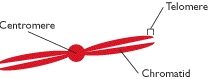
Eukaryotic organelle genomes:
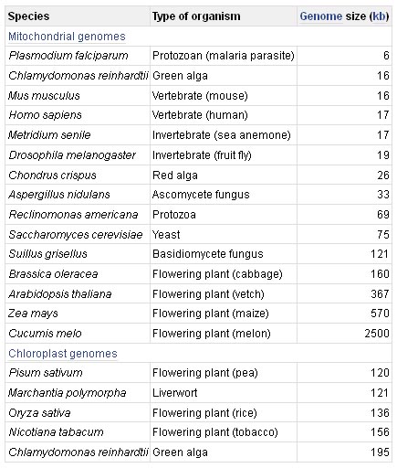
Almost all eukaryotes have mitochondrial genomes, and all photosynthetic eukaryotes have chloroplast genomes. Initially, it was thought that virtually all organelle genomes were circular DNA molecules. Electron microscopy studies had shown both circular and linear DNA in some organelles, but it was assumed that the linear molecules were simply fragments of circular genomes that had become broken during preparation for electron microscopy. We still believe that most mitochondrial and chloroplast genomes are circular, but we now recognize that there is a great deal of variability in different organisms. In many eukaryotes the circular genomes coexist in the organelles with linear versions and, in the case of chloroplasts, with smaller circles that contain subcomponents of the genome as a whole. The latter pattern reaches its extreme in the marine algae called dinoflagellates, whose chloroplast genomes are split into many small circles, each containing just a single gene). We also now realize that the mitochondrial genomes of some microbial eukaryotes (e.g. Paramecium, Chlamydomonas and several yeasts) are always linear.
Copy numbers for organelle genomes are not particularly well understood. Each human mitochondrion contains about 10 identical molecules, which means that there are about 8000 per cell, but in S. cerevisiae the total number is probably smaller (less than 6500) even though there may be over 100 genomes per mitochondrion. Photosynthetic microorganisms such as Chlamydomonas have approximately 1000 chloroplast genomes per cell, about one-fifth the number present in a higher plant cell. One mystery, which dates back to the 1950s and has never been satisfactorily solved, is that when organelle genes are studied in genetic crosses the results suggest that there is just one copy of a mitochondrial or chloroplast genome per cell. This is clearly not the case but indicates that our understanding of the transmission of organelle genomes from parent to offspring is less than perfect.
Mitochondrial genome sizes are variable and are unrelated to the complexity of the organism. Most multicellular animals have small mitochondrial genomes with a compact genetic organization, the genes being close together with little space between them. The human mitochondrial genome, at 16 569 bp, is typical of this type. Most lower eukaryotes such as S. cerevisiae, as well as flowering plants, have larger and less compact mitochondrial genomes, with a number of the genes containing introns.
The endosymbiont theory is based on the observation that the gene expression processes occurring in organelles are similar in many respects to equivalent processes in bacteria. In addition, when nucleotide sequences are compared organelle genes are found to be more similar to equivalent genes from bacteria than they are to eukaryotic nuclear genes. The endosymbiont theory therefore holds that mitochondria and chloroplasts are the relics of free-living bacteria that formed a symbiotic association with the precursor of the eukaryotic cell, way back at the very earliest stages of evolution.
Anatomy of Prokaryotic genomes:
Most prokaryotic genomes are less than 5 Mb in size, although a few are substantially larger than this: B. megaterium, for example, has a huge genome of 30 Mb. The traditional view has been that in a typical prokaryote the genome is contained in a single circular DNA molecule, localized within the nucleoid - the lightly staining region of the otherwise featureless prokaryotic cell. This is certainly true for E. coli and many of the other commonly studied bacteria. However, as we will see, our growing knowledge of prokaryotic genomes is leading us to question several of the preconceptions that became established during the pre-genome era of microbiology. These preconceptions relate both to the physical structure of the prokaryotic genome and its genetic organization.
As with eukaryotic chromosomes, a prokaryotic genome has to squeeze into a relatively tiny space (the circular E. coli chromosome has a circumference of 1.6 mm whereas an E. coli cell is just 1.0 × 2.0 μm) and, as with eukaryotes, this is achieved with the help of DNA-binding proteins that package the genome in an organized fashion. The resulting structure has no substantial similarities with a eukaryotic chromosome, but we still use ‘bacterial chromosome’ as a convenient term to describe it.
Most of what we know about the organization of DNA in the nucleoid comes from studies of E. coli. The first feature to be recognized was that the circular E. coli genome is supercoiled. Supercoiling occurs when additional turns are introduced into the DNA double helix (positive supercoiling) or if turns are removed (negative supercoiling). With a linear molecule, the torsional stress introduced by over- or under-winding is immediately released by rotation of the ends of the DNA molecule, but a circular molecule, having no ends, cannot reduce the strain in this way. Instead the circular molecule responds by winding around itself to form a more compact structure. Supercoiling is therefore an ideal way to package a circular molecule into a small space. Evidence that supercoiling is involved in packaging the circular E. coli genome was first obtained in the 1970s from examination of isolated nucleoids, and subsequently confirmed as a feature of DNA in living cells in 1981. In E. coli, the supercoiling is thought to be generated and controlled by two enzymes, DNA gyrase and DNA topoisomerase I.
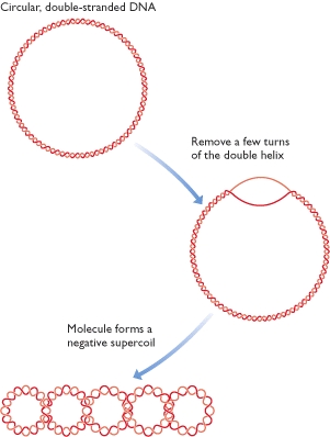
A plasmid is a small piece of DNA, often, but not always circular, that coexists with the main chromosome in a bacterial cell. Some types of plasmid are able to integrate into the main genome, but others are thought to be permanently independent. Plasmids carry genes that are not usually present in the main chromosome, but in many cases these genes are non-essential to the bacterium, coding for characteristics such as antibiotic resistance, which the bacterium does not need if the environmental conditions are amenable. As well as this apparent dispensability, many plasmids are able to transfer from one cell to another, and the same plasmids are sometimes found in bacteria that belong to different species. These various features of plasmids suggest that they are independent entities and that in most cases the plasmid content of a prokaryotic cell should not be included in the definition of its genome.
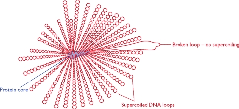
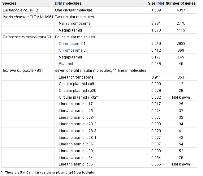
Comparative genomics
Understanding the genome sequence is a massive task that will engage many groups around the world, making use of various techniques and approaches which will be described in the next chapter. Important among these are the use of comparative genomics, in which two complete genome sequences are compared in order to identify common features that, being conserved, are likely to be important. Comparative genomics is a research strategy that uses information obtained from the study of one genome to make inferences about the map positions and functions of genes in a second genome. The basis of comparative genomics is that the genomes of related organisms are similar.
Two organisms with a relatively recent common ancestor will have genomes that display species-specific differences built onto the common plan possessed by the ancestral genome. The closer two organisms are on the evolutionary scale, the more related their genomes will be. If the two organisms are sufficiently closely related then their genomes might display synteny, the partial or complete conservation of gene order. Then it is possible to use map information from one genome to locate genes in the second genome. At one time it was thought that mapping the genomes of the mouse and other mammals, which are at least partially syntenic with the human genome, might provide valuable information that could be used in construction of the human genome map. The problem with this approach is that all the close relatives of humans have equally large genomes that are just as difficult to study, the only advantage being that a genetic map is easier to construct with an animal which, unlike humans, can be subjected to experimental breeding programs. Despite the limitations of human pedigree analysis, progress has been more rapid in mapping the human genome than in mapping those of any of our close relatives, so in this respect comparative genomics is proving more useful in mapping the animal genomes rather than our own. This in itself is a useful corollary to the Human Genome Project because it is revealing animal homologs of human genes involved in diseases, providing animal models for the study of these diseases.
Mapping is significantly easier with a small genome than with a large one. This means that if one member of a pair of syntenic genomes is substantially smaller than the other, then mapping studies with this small genome are likely to provide a real boost to equivalent work with the larger genome. The pufferfish, Fugu rubripes, has been proposed in this capacity with respect to the human genome. The pufferfish genome is just 400 Mb, less than one-seventh the size of the human genome but containing approximately the same number of genes. The mapping work carried out to date with the pufferfish indicates that there is some similarity with the human gene order, at least over short distances. This means that it should be possible, to a certain extent, to use the pufferfish map to find human homologs of pufferfish genes, and vice versa. This may be useful in locating undiscovered human genes, but holds greatest promise in identifying essential sequences such as promoters and other regulatory signals upstream of human genes. This is because these signals are likely to be similar in the two genomes, and recognizable because they are surrounded by non-coding DNA that has diverged quite considerably by random mutations.
One area where comparative genomics has a definite advantage is in the mapping of plant genomes. Wheat provides a good example. Wheat is the most important food plant in the human diet, being responsible for approximately 20% of the human calorific intake, and is therefore one of the crop plants that we most wish to study and possibly manipulate in the quest for improved crops. Unfortunately, the wheat genome is huge at 16 000 Mb, five times larger than even the human genome. A small model genome with a gene order similar to that of wheat would therefore be useful as a means of mapping desirable genes which might then be obtained from their equivalent positions in the wheat genome. Wheat, and other cereals such as rice, are members of the Gramineae, a large and diverse family of grasses. The rice genome is only 430 Mb, substantially smaller than that of wheat, and there are probably other grasses with even smaller genomes. Comparative mapping of the rice and wheat genomes has revealed many similarities, and the possibility therefore exists that genes from the wheat genome might be isolated by first mapping the positions of the equivalent genes in a smaller Gramineae genome.
One of the main reasons for sequencing the human genome is to gain access to the sequences of genes involved in human disease. The hope is that the sequence of a disease gene will provide an insight into the biochemical basis of the disease and hence indicate a way of preventing or treating the disease. Comparative genomics has an important role to play in the study of disease genes because the discovery of a homolog of a human disease gene in a second organism is often the key to understanding the biochemical function of the human gene. If the homolog has already been characterized then the information needed to understand the biochemical role of the human gene may already be in place; if it has not been characterized then the necessary research can be directed at the homolog.
To be useful in the study of disease-causing genes, the second genome does not need to be syntenic with the human genome, nor even particularly closely related. Drosophila holds great promise in this respect, as the phenotypic effects of many Drosophila genes are well known, so the data already exist for inferring the mode of action of human disease genes that have homologs in the Drosophila genome. But the greatest success has been with yeast. Several human disease genes have homologs in the S. cerevisiae genome. These disease genes include ones involved in cancer, cystic fibrosis, and neurological syndromes, and in several cases the yeast homolog has a known function that provides a clear indication of the biochemical activity of the human gene. In some cases it has even been possible to demonstrate a physiological similarity between the gene activity in humans and yeast. For example, the yeast gene SGS1 is a homolog of a human gene involved in the diseases called Bloom's and Werner's syndromes, which are characterized by growth disorders. Yeasts with a mutant SGS1 gene live for shorter periods than normal yeasts and display accelerated onset-of-aging indicators such as sterility. The yeast gene has been shown to code for one of a pair of related DNA helicases that are required for transcription of rRNA genes and for DNA replication. The link between SGS1 and the genes for Bloom's and Werner's syndromes, provided by comparative genomics, has therefore indicated the possible biochemical basis of the human diseases.
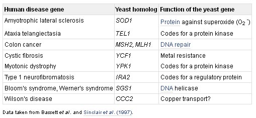
Homologous genes are ones that share a common evolutionary ancestor, revealed by sequence similarities between the genes.
· Orthologous genes are those homologs that are present in different organisms and whose common ancestor predates the split between the species.
· Paralogous genes are present in the same organism, often members of a recognized multigene family, their common ancestor possibly or possibly not predating the species in which the genes are now found.
A pair of homologous genes do not usually have identical nucleotide sequences, because the two genes undergo different random changes by mutation, but they have similar sequences because these random changes have operated on the same starting sequence, the common ancestral gene. Homology searching makes use of these sequence similarities. The basis of the analysis is that if a newly sequenced gene turns out to be similar to a previously sequenced gene, then an evolutionary relationship can be inferred and the function of the new gene is likely to be the same, or at least similar, to the function of the known gene.
It is important not to confuse the words homology and similarity. It is incorrect to describe a pair of related genes as ‘80% homologous’ if their sequences have 80% nucleotide identity. A pair of genes are either evolutionarily related or they are not; there are no in-between situations and it is therefore meaningless to ascribe a percentage value to homology.
Full genome alignment
Genome sequence alignments are a priceless resource for finding functional elements (protein-coding sequences, RNA structures, cis-regulatory elements, miRNA target sites, etc.) and charting evolutionary history. Many genome alignment algorithms have been developed. All of these algorithms require selection of various mundane but critical parameters. In the most classic approach to alignment (Smith-Waterman/BLAST), these parameters include the scoring matrix and gap costs, which determine alignment scores, and thus which alignments are produced. Five important parameters of full genome alignment are as follows:
alignment score cutoff
In the classic alignment framework, it is necessary to choose an alignment score cutoff: low enough to find weak homologies, but high enough to avoid too many spurious alignments. A rational approach is to calculate the E-value--the expected number of alignments between two random sequences scoring above the cutoff--and choose a cutoff that has an acceptable E-value.
Repeat masking
There is a general awareness that repeat-masking is important for genome alignment, but the efficacy of repeat-masking methods has not been assessed in this context. "Repeats" can be categorized into two types: simple (low entropy) sequences such as ATATATATAT, and non-simple repeats such as Alu elements. Simple repeats cause spurious (i.e. non-homologous) alignments with high scores, but non-simple repeats do not, because e.g. every Alu is genuinely homologous to every other Alu. Non-simple repeats cause a different problem: too many alignments.
Scoring matrix
The scoring matrix specifies a score for aligning every kind of base with every other kind of base. The simplest scoring matrix, which is actually quite good for DNA, is: +1 for all matches and -1 for all mismatches. Given a set of trusted alignments, a scoring matrix is often derived using log likelihood ratios. This is because, under simplifying independence assumptions, log likelihood ratio derived scores are theoretically optimal for discriminating between random and true alignments.
Gap costs
Effective gap costs for protein alignment have been studied empirically, but not for DNA alignment.
X-drop parameter
BLAST and similar methods, including BLASTZ and LAST, have an important but rarely considered X-drop parameter. (In NCBI BLAST and LAST this parameter is called "X", but in BLASTZ it is called "Y".) When extending gapped alignments, these methods terminate the extension when the score drops by more than X below the maximum previously seen. This serves two purposes: to reduce computation time, and to prevent spurious internal regions in alignments. Without any X-drop criterion, maximum-score alignments can contain arbitrarily poor internal segments. Thus the X-drop parameter is not merely an algorithmic detail: it is one of the parameters that define what a good alignment is.
Base level security
Sequence alignments are inherently uncertain. This uncertainty has traditionally been disregarded, leading to errors in many kinds of inferences made from alignments. Fortunately, it is possible to quantify this uncertainty, by estimating an alignment probability for every possible pair of aligned bases. We have made it easy to obtain these probabilities, by integrating their calculation into our alignment software, LAST. Below, we confirm that they are useful for measuring reliability and controlling the sensitivity/specificity tradeoff at the level of aligned bases.
Recent progress in whole genome shotgun sequencing and assembly technologies has drastically reduced the cost of decoding an organism's DNA, which has resulted in a rapid increase in genomic sequencing projects. According to the Genomes OnLine Database v2.0, as of August 2006 there are over 2000 active genome sequencing projects, including 413 that have already been completed and published. Of the remaining unpublished projects, there are nearly 1000 ongoing bacterial genome sequencing projects. This high concentration of bacterial genomes currently being sequenced will soon provide access to several genomes of closely related species. In fact, the Bacillus species alone will soon increase from 13 published genomes to 57 through active sequencing projects. Additionally, the Yersinia and Salmonella species, both will soon grow from 6 and 5 published genomes, to 22 and 23, respectively. This trend follows with E. Coli and Burkholderia species, each soon to increase from 7 to 35, and, 7 to 44 published genomes. This increase in closely related DNA sequence will allow for in depth studies of closely related species through multiple whole genome comparisons.
Multiple genome comparison helps to identify biological similarities and differences in a set of genomes at the nucleotide level, identifying genomic regions that may have been conserved among several organisms. This information then can be used to make inferences about phylogeny, functional regions, and gene predictions. Figure offers an approximate, and by no means complete, overview of the landscape of global comparison and alignment tools over the last 30 years.
Comparison of large genomes
Multiple genome comparison tools need to be able to efficiently handle comparisons involving megabases of genomic sequence. However, large-scale sequence alignment does not come cheap. Using traditional methods, obtaining an optimal global alignment between two sequences with more than 10,000 nt can be computationally expensive, requiring days or even months of computation time, even on well equipped computers. Thus, the first classification level in Figure 1 separates those tools able to efficiently handle small (< 10, 000 nt) or large (≥ 10, 000 nt) sequence comparisons through alignment.
Comparison of multiple genomes
Multiple genome alignments provide for rich and sensitive comparisons that are able to identify small regions that may have been conserved or evolved among several organisms. The problem of multiple sequence alignment, however, is not in its utility but rather its complexity. Performing optimal multiple sequence alignment via dynamic programming requires O(LN) time and space complexity, where L is the length of the sequence and N the number of sequences involved in the multiple alignment. This severely limits the number of genomes able to efficiently compared and aligned using such methods, which is our next classification level for the comparative genomics tools.
Comparison of closely related genomes
Due to the rapid growth in published genomic sequence, several closely related species comparisons will soon be possible. Recent progress in progressive alignment methods have allowed for thorough and accurate comparisons even among distantly related species. While they offer high sensitivity when comparing multiple, distantly related species, such as human and fish, and avoid the reference sequence limitation, these tools require a quadratic number of pairwise global comparisons and can quickly become computationally expensive when comparing several large genomes. When certain assumptions can be made about the set of genomes being compared, such as the overall level of sequence similarity, alternative techniques can be used to perform simultaneous detection of matching regions in all of the genomes being compared. Methods based on multi-MUMs or multi-MEMs achieve exactly this, and are able to compare multiple, large genomes in a fraction of the time, allowing for more efficient and interactive genome comparisons. The third level of classification then separates those tools that were originally designed accurately compare and align large, multiple genomes using progressive alignment methods from those that have assumed some level of sequence conservation in the input sequences for rapid comparisons of closely related species.
Comparisons involving rearrangements
Rearrangements can cause major variations in gene order and content among closely related organisms. Bacterial genomes often are full of rearrangements, or disorder and large-scale inversions in bacteria were first reported. For accurate genome comparisons, it is then essential to correctly identify and track these shuffled regions to ensure an accurate global comparison of multiple bacterial genomes. As a final classification level, we distinguish between methods able to detect shuffled or rearranged similarity, such as transpositions or inversions, in multiple closely related species with large genomes from those that assume collinearity.
The challenges of whole genome alignment
The standard algorithms for sequence alignment rely on either dynamic programming or hashing techniques. Naïve versions of dynamic programming use O(n2) space and time (where n is the length of the shorter of the two sequences being compared), which makes computation simply unfeasible for sequences of size ≥4 Mb (such as the two M.tuberculosis genomes). [For an input with size n, a function X is O(n2) if, for sufficiently large n and for some constant C independent of n, X ≤ C·n2. Informally stated, the O(n2) notation means that the amount of space and time required for the computation is no more than Cn2.] Hashing techniques operate faster on average, but they involve a ‘match and extend’ strategy, where the ‘extend’ part also takes O(n2) time. For dynamic programming, it is possible to reduce the required space to O(n) by taking more time; this solves the memory problem but still leaves one with an unacceptably slow algorithm. Faster algorithms can be developed for specialized purposes, such as a recent system for finding tandem repeats. This repeat finder uses a k-tuple hashing algorithm and couples it with a stochastic pattern matching strategy.
More complex dynamic programming methods can be used for alignment when the alignment error is expected to be low. For example, one can align two similar sequences with at most E differences (or errors) in time proportional to E times the length of the longer sequence. The sim3 program uses a linear time algorithm that works well when the input sequences are highly similar; it runs very fast even on very long sequences. Unfortunately, this class of algorithms does not always work for whole genome alignments, since the ‘errors’ may include multiple large inserts on the order of 104 or 105 nucleotides. As we demonstrate below, the number of differences may be greater than 100 000 despite the fact that the genomes (in this case M.genitalium and M.pneumoniae) are closely related and can in fact be aligned with one another.
Another system developed to align long sequences is sim2. This system uses a BLAST-like hashing scheme to identify exact k-mer matches, which are extended to maximal-length matches. These maximal matches are then combined into local alignment chains by a dynamic programming step. In contrast, our suffix-tree approach directly finds maximal matches that are unique. These matches can then be easily ordered to form the basis of an alignment that can span even very long mismatch regions between the two input genomes.
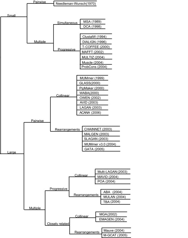
Algorithms:
Finding the orthologous regions between two species computationally is a nontrivial task that has never been explored on a whole-genome scale for vertebrate genomes.
Local alignment tools find many high-scoring matching segments, in particular the orthologous segments, but in addition they identify many paralogous relationships, or even false-positive alignments resulting from simple sequence repeats and other sequence artifacts (Chen et al. 2001). BLAST was successfully utilized in the study by Gibbs and coauthors (Chen et al. 2001) where high-quality rat WGS reads (covering 7.5% of the rat genome) were compared with the GoldenPath human genome assembly. Those authors investigated statistical significance of BLAST search results and parameters, but they did not focus on finding ‘true’ orthologs and were mostly interested in higher sensitivity of alignment and completeness of coverage of coding exons. When compared with the human assembly, more than 47.3% of all aligned reads produced between two and 12 hits (which correspond to medium represented elements), and 7.6% had more than 12 hits (likely containing repetitive elements).
Unlike local alignment, global alignment methods require aligned features to be conserved in both order and orientation, and are therefore appropriate for aligning orthologous regions in the domain where this assumption applies. But whole-genome rearrangements, duplications, inversions, and other evolutionary events restrict the resolution at which the order and orientation assumption of global alignment applies. In the case of the human and mouse genomes, it appears that this assumption applies, on average, to regions less than eight megabases in length (Mural et al. 2002).
Our strategy is to use a fast local alignment method to find anchors on the base genome to identify regions of possible homology for a query sequence. The key element is then to be able to postprocess these anchors in order to delimit a region of homology where the order and orientation seem conserved. These regions are then globally aligned. In the work presented here, we used BLAT (Kent 2002) to find anchors and AVID (version 2.0 at http://bio.math.berkeley.edu/avid; Bray et al. 2003) to generate global alignments for an overview of the pipeline and how they were combined). BLAT was designed for cDNA/DNA alignment and first used in Intronerator (Kent and Zahler 2000). BLAT is not optimized for cross-species alignments (Kent 2002), but we chose this program because our tests demonstrated that it performed very well as an anchoring tool in our computational scheme. It is also about 500 times faster than other existing alignment tools.
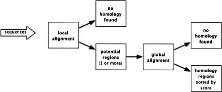
For each sequence, BLAT matches are sorted by score, and regions of possible homology are selected around the strongest matches which serve as anchors. All BLAT hits at most L bases apart are grouped together (here L is the length of the region being aligned). For groups smaller than L/4, the regions were then extended out by min(50k, L/2-–G) where G is the length of the group. For groups with G greater than L/4, the regions were extended out by min(50k,L/4). The groups obtained are compared and the ones with less than 30% of the score of the best group are rejected at this stage. Various parameters for these heuristics were explored in order to obtain a method that would work for different sizes of sequences.
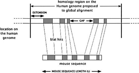
This heuristic may identify multiple regions of possible homology of different size and score in the base genome. These regions are proposed as candidates to the alignment program. The score obtained by the global alignment is used to make the decision about which alignments to report or to reject.
MUMmer
MUMmer is an open source software package for the rapid alignment of very large DNA and amino acid sequences. The latest version, release 3.0, includes a new suffix tree algorithm that has further improved the efficiency of the package and has been integral to making MUMmer an open source product.
MUMmer is a
modular and versatile package that relies on a suffix tree data structure for
efficient pattern matching. Suffix trees are suited for large data sets because
they can be constructed and searched in linear time and space. This allows
mummer
to find all 20 base pair maximal exact matches between two ~5 million base pair
bacterial genomes in 20 seconds, using 90 MB of RAM, on a typical 1.7 GHz Linux
desktop computer. Using a seed and extend strategy, other parts of the MUMmer
pipeline use these exact matches as alignment anchors to generate pair-wise
alignments similar to BLAST output. Also included are some utilities to handle
the alignment output and a primitive plotting tool (mummerplot)
that allows the user to convert MUMmer output to
gnuplot files for
dot and percent identity plots. Another graphical utility called MapView is
included with the MUMmer distribution and displays sequence alignments to a
annotated reference sequence for exon refinement and investigation.
This modular design has an important side effect, it allows for the easy reuse of MUMmer modules in other software. For instance, one can imagine primer design, repeat masking and even comparative annotation tools based on the efficient matching algorithm MUMmer provides. Another advantage of MUMmer is its speed. Its low runtime and memory requirements allow it to be used on most any computer. MUMmer's efficiency also makes it ideal for aligning huge sequences such as completed and draft eukarotic genomes. MUMmer has been successfully used to align the mouse and human genomes, showing it can handle most any input available. In addition, its ability to handle multiple sequences facilitate many vs. many searches, and make the comparison of unfinished draft sequence quite simple. However, because of it's many abilities, inexperienced users may find it difficult to determine the best methods for their application, so please refer to the Running MUMmer and Use cases sections for brief descriptions, use case examples, and tips on making the most of the MUMmer package, or if you want to understand more about a specific utility, refer to Program descriptions section for more detailed information and output formats.
The five most
commonly used programs in the MUMmer package are
mummer,
nucmer,
promer,
run-mummer1
and
run-mummer3,
so this section covers the basics of executing these tools and what each of them
specializes in. To better understand how to view the outputs of these programs,
please refer to the use cases section or the MUMmer examples webpage for a brief
walk-through of each major module with full input data and expected outputs. For
further information, please refer to the Program descriptions section for a
detailed explanation of each program and its output.
Mummer Package
The MUMmer package provides efficient means for comparing an entire genome against another. However, until 1999 there were no two genomes of sufficient similarity to compare. With the publication of the second strain of Helicobacter pylori in 1999, following the publication of the first strain in 1997, the scientific world had its first chance to look at two complete bacterial genomes whose DNA sequences were highly similar. The number of pairs of closely-related genomes has exploded in recent years, facilitating many comparative studies. For instance, the published databases include the following genomes for which multiple strains and/or multiple species have been sequenced:
Human vs Human
With the capability to align the entire human genome to itself, there is no genome too large for MUMmer. The following table gives run times and space requirements for a cross comparison of all human chromosomes. The 1st column indicates the chromosome number, with "Un" referring to unmapped contigs. Column 2 shows chromosome length and column 4 shows the length of the total genomic DNA searched against the chromosome in column 1. Column 3 shows the time to construct the suffix tree, and column 5 the time to stream the query sequence through it. Column 6 shows the maximum amount of computer memory occupied by the program and data, and column 7 shows memory usage for the suffix tree in bytes per base pair. Each human chromosome was used as a reference, and the rest of the genome was used as a query and streamed against it. To avoid duplication, we only included chromosomes in the query if they had not already been compared; thus we first used chromosome 1 as a reference, and streamed the other 23 chromosomes against it. Then we used chromosome 2 as a reference, and streamed chromosomes 3–22, X, and Y against that, and so on.
mummer
is a suffix tree algorithm designed to find maximal exact matches of some
minimum length between two input sequences. MUMmer's namesake program originally
stood for Maximal Unique Matcher, however in
subsequent versions the meaning of
unique has been
skewed. The original version (1.0) required all maximal matches to be unique in
both the reference and the query sequence (MUMs); the second version (2.0)
required uniqueness only in the reference sequence (MUM-candidates); and the
current version (3.0) can ignore uniqueness completely, however it defaults to
finding MUM-candidates and can be switched on the command line. To restate, by
default
mummer
will only find maximal matches that are unique in the entire set of reference
sequences. The match lists produced by
mummer
can be used alone to generate alignment dot plots, or can be passed on to the
clustering algorithms for the identification of longer non-exact regions of
conservation. These match lists have great versatility because they contain huge
amounts of information and can be passed forward to other interpretation
programs for clustering, analysis, searching, etc.
mummer
achieves its high performance by using a very efficient data structure known as
a suffix tree. This data structure can be both constructed and searched in
linear time, making it ideal for large scale pattern matching. To save memory,
only the reference sequence(s) is used to construct the suffix tree and the
query sequences are then streamed through the data structure while all of the
maximal exact matches are extracted and displayed to the user. Because only the
reference sequence is loaded into memory, the space requirement for any
particular
mummer
run is only dependent on the size of the reference sequence. Therefore, if you
have a reasonably sized sequence set that you want to match against an enormous
set of sequences, it is wise to make the smaller file the reference to assure
the process will not exhaust your computer's memory resources. The query files
are loaded into memory one at a time, so for an enormous query that will require
a significant amount of memory just to load the character string, it is helpful
to partition the query into multiple smaller files using the syntax.
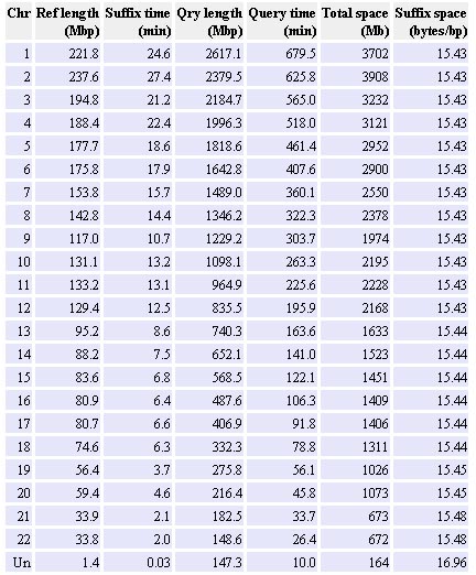
Algorithms:
The basis of the algorithm is a data structure known as a suffix tree, which allows one to find, extremely efficiently, all distinct subsequences in a given sequence. The first efficient algorithms to construct suffix trees were given by Weiner and McCreight, and this data structure has been studied extensively for more than two decades. For the task of comparing two DNA sequences, suffix trees allow us to quickly find all subsequences shared by the two inputs. The alignment is then built upon this information.
Our system uses a combination of three ideas: suffix trees, the longest increasing subsequence (LIS) and Smith-Waterman alignment. The novelty of the system derives from the integration of these ideas into a coherent system for large-scale genome alignment.
The inputs to the system are two sequences, which for convenience we refer to as Genome A and Genome B. Note that any sequences can be provided as input (in fact, we have a modified version of the system that handles protein sequences), but we will use DNA for the purposes of discussion. We assume the sequences to be compared are closely homologous. In particular, we assume that there is a mapping between large subsequences of the two inputs, presumably because they evolved from a common ancestor. The main biological features that the system identifies are as follows. (i) SNPs, defined here as a single mutation ‘surrounded’ by two matching regions on both sides of the mutation. (ii) Regions of DNA where the two input sequences have diverged by more than an SNP. (iii) Large regions of DNA that have been inserted into one of the genomes, for example by transposition, sequence reversal or lateral transfer from another organism. (iv) Repeats, usually in the form of a duplication that has occurred in one genome but not the other. The repeated regions can appear in widely scattered locations in the input sequences. (v) Tandem repeats, regions of repeated DNA that might occur in immediate succession, but with different copy numbers in the two genomes. The copy numbers do not have to be integers; e.g., a repeat could occur 2.5 times in one genome and 4.2 times in the other.
The alignment process consists of the following steps, which are described in more detail in subsequent sections.
(i) Perform a maximal unique match (MUM) decomposition of the two genomes. This decomposition identifies all maximal, unique matching subsequences in both genomes. An MUM is a subsequence that occurs exactly once in Genome A and once in Genome B, and is not contained in any longer such sequence. Thus, the two character positions bounding an MUM must be mismatches, as shown in Figure. The crucial principle behind this step is the following: if a long, perfectly matching sequence occurs exactly once in each genome, it is almost certain to be part of the global alignment. (Note that a similar intuition is behind the hashing method upon which FASTA and BLAST are based.) Thus, we can build the global alignment around the MUM alignment. Because of the assumption that the two genomes are highly similar, we are assured that a large number of MUMs will be identified.
MUMs on both DNA strands are identified; this allows the system to identify sequences from one genome that appear reversed in the other genome.
(ii) Sort the matches found in the MUM alignment, and extract the longest possible set of matches that occur in the same order in both genomes. This is done using a variation of the well-known algorithm to find the LIS of a sequence of integers. Thus, we compute an ordered MUM alignment that provides an easy and natural way to scan the alignment from left to right.
(iii) Close the gaps in the alignment by performing local identification of large inserts, repeats, small mutated regions, tandem repeats and SNPs.
(iv) Output the alignment, including all the matches in the MUM alignment as well as the detailed alignments of regions that do not match exactly.
The system, which is called MUMmer, is packaged as three independent modules: suffix tree construction, sorting and extraction of the LIS, and generation of Smith-Waterman alignments for all the regions between the MUMs. The last step can easily be replaced with another alignment program if a user wishes.
![]()
Figure: A maximal unique matching subsequence (MUM) of 39 nt (shown in uppercase) shared by Genome A and Genome B. Any extension of the MUM will result in a mismatch. By definition, an MUM does not occur anywhere else in either genome.
Figure: Suffix tree for the sequence gaaccgacct. Square nodes are leaves and represent complete suffixes. They are labeled by the starting position of the suffix. Circular nodes represent repeated sequences and are labeled by the length of that sequence. In this example the longest repeated sequence is acc occurring at positions 3 and 7.
Applications
MUMmer 1 was used to detect numerous large-scale inversions in bacterial genomes, leading to a new model of chromosome inversions, reported in this 2000 Genome Biology paper. It was also used to discover evidence for a recent whole-genome duplication in Arabidopsis thaliana, reported in "Analysis of the genome sequence of the flowering plant Arabidopsis thaliana." The Arabidopsis Genome Initiative, Nature 408 (2000), 796-815.
MUMmer 2 was used to align all human chromosomes to one another and to detect numerous large-scale, ancient segmental duplications in the human genome, as reported in "The sequence of the human genome." Venter et al., Science 291 (2001), 1304-1351. PROmer was used to compare the human and mouse malaria parasites P.falciparium and P.yoelii, as described in "Genome sequence and comparative analysis of the model rodent malaria parasite Plasmodium yoelii yoelii." J.M. Carlton et al., Nature 419 (2002), 512-519.
MUMmer 3 is the latest version, and is downloaded roughly 300 times every month. That's over 7,000 users in the 2 years after its release. In addition, the three versions of MUMmer have a combined citation count of over 700 papers.
Figure: Aligning Genome A and Genome B after locating the MUMs. Each MUM is here indicated only by a number, regardless of its length. The top alignment shows all the MUMs. The shift of MUM 5 in Genome B indicates a transposition. The shift of MUM 3 could be simply a random match or part of an inexact repeat sequence. The bottom alignment shows just the LIS of MUMs in Genome B.
MegaBLAST
MegaBLAST uses the greedy algorithm of Webb Miller et al. for nucleotide sequence alignment search and concatenates many queries to save time spent scanning the database. It is up to ten times faster than more common sequence similarity programs and therefore can be used to swiftly compare two large sets of sequences against each other.
For aligning DNA sequences that differ only by sequencing errors, or by equivalent errors from other sources, a greedy algorithm can be much faster than traditional dynamic programming approaches and yet produce an alignment that is guaranteed to be theoretically optimal.
The best way to identify an unknown sequence is to see if that sequence already exists in a public database. If the database sequence is a well-characterized sequence, then one will have access to a wealth of biological information. MEGABLAST, discontiguous-megablast, and blastn all can be used to accomplish this goal. However, MEGABLAST is specifically designed to efficiently find long alignments between very similar sequences and thus is the best tool to use to find the identical match to your query sequence. In addition to the expect value significance cut-off, MEGABLAST also provides an adjustable percent identity cut-off for the alignment, which provides cut-off in addition to the significance cut-off threshold set by Expect value.
The BLAST
nucleotide algorithm finds similar sequences by breaking the query into short
subsequences called words. The program identifies the exact matches to the query
words first (word hits). BLAST program then extends these word hits in multiple
steps to generate the final gapped alignments.
One of the important parameters governing the sensitivity of BLAST searches is
the length of the initial words, or word size as it is called. The most
important reason that blastn is more sensitive than MEGABLAST is that it uses a
shorter default word size (11). Because of this, blastn is better than MEGABLAST
at finding alignments to related nucleotide sequences from other organisms. The
word size is adjustable in blastn and can be reduced from the default value to a
minimum of 7 to increase search sensitivity.
A more sensitive search can be achieved by using the newly introduced
discontiguous megablast page. This page uses an algorithm with the same name,
which is similar to that reported by Ma et.al. Rather than requiring
exact word matches as seeds for alignment extension, discontiguous megablast
uses non-contiguous word within a longer window of template. In coding mode, the
third base wobbling is taken into consideration by focusing on finding matches
at the first and second codon positions while ignoring the mismatches in the
third position. Searching in discontiguous MEGABLAST using the same word size is
more sensitive and efficient than standard blastn using the same word size. For
this reason, it is now the recommended tool for this type of search. Alternative
non-coding patterns can also be specified if desired. Additional details on
discontiguous are available at:www.ncbi.nlm.nih.gov/Web/Newsltr/FallWinter02/blastlab.html.
Parameters unique for discontiguous megablast are:
It is important to point out that nucleotide-nucleotide searches are not the best method for finding homologous protein coding regions in other organisms. That task is better accomplished by performing searches at the protein level, by direct protein-protein BLAST searches or by translated BLAST searches. This is because of the codon degeneracy, the greater information available in amino acid sequence, and the more sophisticated algorithm and scoring matrix used in protein-protein BLAST.
MegaBlast takes as input a set of FASTA formatted DNA query sequences. These can be either pasted into a provided text area, or downloaded from a file. It is preferrable to submit many query sequences at a time, but not more than 16383. The algorithm concatenates all the query sequences together and performs search on thus obtained long single sequence. After the search is done, the results are re-sorted by query sequence. The database input for MegaBlast is any "blastable" database, obtained from the ftp server or via formatdb program from a FASTA formatted file.
Unlike BLAST, MegaBlast is most efficient in both speed and memory requirements with non-affine gap penalties, i.e. gap opening cost of 0 and gap extension penalty E = match_reward/2 - mismatch_penalty. These values of gapping parameters are default. To set the affine penalties, advanced options should be used. It is not recommended to use the affine version of MegaBlast with large databases or very long query sequences.
-W Word size. Any value of W, that is not divisible by 4, is equivalent to the nearest value divisible by 4 (with 4i+2 equivalent to 4i). When W is divisible by 4, MegaBlast finds any exact match of length W that starts at a position in the database sequence divisible by 4 (count starting from 0). Thus it is guaranteed that all perfect matches of length W + 3 will be found and extended by the MegaBlast search. It is preferrable to use MegaBlast with word sizes at least 12. With word size 8 the algorithm becomes much slower. All other advanced options have the same meaning as in regular BLAST.
Greedy Algorithm
Greedy alignment algorithms work directly with a measurement of the difference between two sequences, rather than their similarity. In other words, near-identity of sequences is characterized by a small positive number instead of a large one. In the simplest approach, an alignment is assessed by counting the number of its differences, i.e., the number of columns that do not align identical nucleotides. The distance, D(i, j), between the strings a1a2 . . . ai and b1b2 . . . b j is then de. ned as the minimum number of differences in any alignments of those strings.
We will need the ability to translate back and forth between an alignment’s score and the number of its differences, but this requirement constrains the alignment scoring parameters. Assume for the moment that any two alignments of a1a2 . . . ai and b1b2 . . . bj having the same number of differences also have the same score, regardless of the particular sequence entries. Pick any such alignment that has at least two mismatch columns. One of those columns can be replaced by a deletion column followed by an insertion and, by changing one of the sequence entries, the other mismatch can be converted to a match. The transformation can be pictured as:
Here, dots mark alignment entries that are unchanged between the two alignments. This transformation leaves the number of differences, and hence the score, unchanged, from which it follows that 2 X mis = 2 X ind + mat. In summary, the equivalence of score and distance implies that ind = mis – mat/2. As the following lemma shows, that equality is sufficient to guarantee the desired equivalence and, furthermore, the formula to translate distance into score depends only on the antidiagonal containing the alignment end-point.
Lemma 1. Suppose the alignment scoring parameters satisfy ind = mis – mat/2. Then any alignment
of a1a2 . . . ai and b1b2 . . . b j with d differences has score S’(i + j, d) = (i + j )Xmat/2 - d X (mat-¡ mis).
Proof. Consider such an alignment with J matches, K mismatches and I indels, and let k = i +j. Then k = 2J + 2K + I, since each match or mismatch extends the alignment for two antidiagonals, while each indel extends it by one. The alignment has d = K + I differences, while its similarity score is
mat X J + mis X K + ind X I = mat X (k - 2K - I) / 2 + mis X K + (mis - mat/2) X I
= k X mat/2 - d X (mat - mis).
For the remainder of this section, we assume that ind = mis - mat/2. Rather than determining values S(i, j) in order of increasing antidiagonal, the values will be found in order of increasing D(i, j ). Note that Lemma 1 implies that minimizing the number of differences in an alignment is equivalent to maximizing its score (for a fixed point (i, j)), and that S(i, j) = S’(i + j, D(i, j)). In brief, knowing D(i, j ) immediately tells us S(i, j).
The points where D equals 0 are just the (i, i ) where ap = bp for all p ≤ i, since for other (i, j) an alignment of a1a2 . . . ai and b1b2 . . . b j must contain at least one replacement or indel. Ignoring for the moment the X-drop condition, suppose we have determined all positions (i, j ) where D(i, j) = d- 1. In particular, suppose we know the values R(d- 1, k) giving the x -coordinate of the last position on diagonal k where the D-value is d - 1, for – d< k< d. (The kth diagonal consists of the points (i, j) where i- j= k.) Note that if D(i, j) , d, then (i, j) is on diagonal k with |k|< d.
Consider any (i, j) on diagonal k and where D(i, j) = d. Pick any alignment of a1a2 . . . ai and b1b2 . . . b j having d differences. Imagine removing columns from the right end of the alignment that consist of a match. In terms of the grid, this moves us down diagonal k toward (0, 0), through points with D-value d. The process stops when we hit a mismatch or indel column. Removing that column takes us to a point with D-value d - 1. We can reverse this process to determine the D-values in diagonal k or, to be more precise, to determine R(d, k), the x -coordinate of the last position in diagonal k where D(i, j) 5 d. Namely, we . nd one position where D(i, j) = d and j = i- k, as illustrated in Figure , then simultaneously increment i and j until ai+11 ≠ b j+ 1.
What remains is to simulate line 12 of Figure 2. That is, we need a way to tell if S(i, j) < T- X , where T is the maximum S( p, q) over all ( p, q) where p + q < i + j. This was easy to do when the S-values were being determined in order of increasing antidiagonal, but now we are determining the S-values in a different order. It will be insuf. cient to simply keep the largest S-value determined so far in the computation, but we can get by with only a little more effort. (Our argument for this depends critically on our use of “half-nodes” in Figure 2.) Let “phase x ” refer to the phase in the greedy algorithm that determines points where D(i, j) = x , and let T [x ] be the largest S-value determined during phases 0 through x .
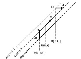
Three cases for finding a point of distance d on diagonal k. The R-values give x -coordinates of the last positions on each diagonal with D-value d - 1. We can move right from a d - 1, or along a diagonal from a d - 1, or up from a d - 1, in order to find a point that can be reached with d differences. The furthest of these points along diagonal k must have D-value d. The first two moves raise the x -coordinate by 1. See line 10 of Figure.
Given the values T [x ] for x<, d, and knowing that D(i, j) = d (and hence that S(i, j) = S’(i + j, d),where S0 is as in Lemma 1), how can we determine the maximum S-value over all points on antidiagonals strictly before i + j? Note that there may well be points in those earlier antidiagonals whose S-value has not yet been determined. However, any such S-value will be smaller than S(i, j ), according to Lemma 1. In fact, any S-value on an earlier antidiagonal that exceeds S(i, j) by more than X must have been determined a number of phases before phase d. The following result makes this precise.
Lemma 2. Suppose D(i, j ) = d, define
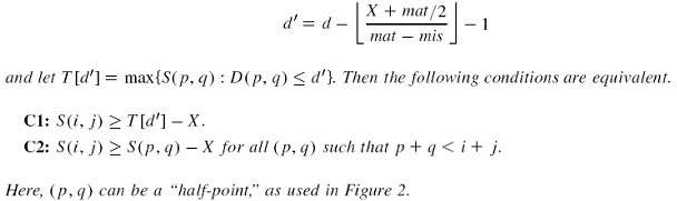
Proof. Our greedy algorithm treats only integer values of d. However, let us de. ne D(i + ½, j + 1/2) to be (D(i, j) + D(i + 1, j + 1))/2, for all integers i , M and j , N . Note that T [d’] is unchanged since d’ is an integer. It is straightforward to verify that the formula for S in terms of D holds for half-points, i.e., S(i + ½, , j+ ½ ) = (i + j + 1)mat/2 - D(i + ½, , j+ ½)(mat - mis). First we show that C1 implies C2 by assuming that C2 is false and proving that C1 is then false. Suppose S( p, q) > S(i, j) + X for some ( p, q) satisfying p + q < i + j. Then
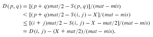
Without loss of generality, D( p, q) is an integer, since otherwise ( p, q) is a half-point on a mismatch edge, and S( p – 1/2, q- 1/2) > S( p, q). Let V denote (X + mat/2)/(mat - mis). Then D(i, j) - D( p, q) is the first integer strictly larger than V (i.e., [V] + 1 or more). Hence D( p, q) ≤ d’. It follows that S(i, j) + X< S( p, q) ≤ T [d’].
For the converse, we assume that C1 is false and prove that C2 is then false. Suppose that S(i, j ) < T [d’] - X . By definition, T [d’] equals some S( p, q) where D( p, q) ≤ d’. If p + q < i+ j, then we’ve found a witness that C2 is false. But what if (p, q)’s antidiagonal is not smaller than (i, j)’s? Then pick an alignment ending at ( p, q) and having at most d’ differences. Consider the initial portion of that alignment ending on antidiagonal i + j - 1, say at ( p’, q’). (This is where half-points may be necessary; without half–points, the antidiagonal index would increase by 2 along match and mismatch edges.) That prefix has at most d0 differences, and hence
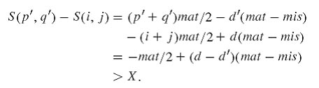
In summary, comparing S(i, j ) with T [d’] - X immediately tells us if S(i, j) should be pruned. Note that this test need only be performed when we . rst . nd a point (i, j) on diagonal k and where D(i, j) = d, since if that point survives, then subsequent points on that diagonal with D-value d have their S-value increasing as fast as possible and hence won’t be pruned. To be precise, suppose S(i, j) ≥ S( p, q) - X for all ( p, q) satisfying p + q < i + j, and let D(i + t, j + t) = D(i, j) for some t > 0. Then S(i + t, j + t)
= S(i, j) + t X mat ≥ S( p, q) - X + t X mat ≥ S( p + t, q+ t) - X for all ( p + t, q + t) such that p + q + 2t , i + j + 2t.
Theorem 1. Assume an alignment-scoring scheme in which ind = mis – mat/2, where mat > 0, mis < 0 and ind < 0 are the scores for a match, mismatch and insertion/deletion, respectively. The algorithm of Figure 4, with S’ as defined in Lemma 1, always computes the same optimal alignment score as does the algorithm of Figure 2.
Proof.
First note
that the previous discussion, including Lemma 2, implies the equivalence of the
algorithms if no pruning is performed (lines 13–16 of Figure 2 and lines 19–22
of Figure 4). But pruning does not affect the computed result. In particular,
consider lines 21–22 of Figure 4, which handle situations when the grid boundary
is reached. If extension down diagonal
k
reaches
i =
M,
then there is no need to consider diagonals larger than
i,
since positions searched at a later phase (larger
d)
will have smaller antidiagonal index, and hence smaller score. Thus we set
U
![]() k
- 2,
so that when diagonals with index at most
U +
1 are considered in the next phase, unnecessary work will be avoided.
L
is handled
similarly.
k
- 2,
so that when diagonals with index at most
U +
1 are considered in the next phase, unnecessary work will be avoided.
L
is handled
similarly.
Let
dmax
and
L
≤
M
+
N
denote the
largest values of
d
and of
i
+
j
attained
when the algorithm of Figure 4 is executed. Then the algorithm’s worst-case
running time is
O
(dmax
L).
The distinction between this algorithm and earlier greedy alignment methods is
that another worst-case bound for the current method is ![]() ,
where
L d
and
Ud
denote the
lower and upper bounds of {k
:
R(d,
k)
> - ∞ }.
,
where
L d
and
Ud
denote the
lower and upper bounds of {k
:
R(d,
k)
> - ∞ }.
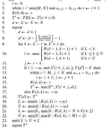
Greedy algorithm that is equivalent to the algorithm of Figure 2 if ind 5 mis ¡ mat=2.
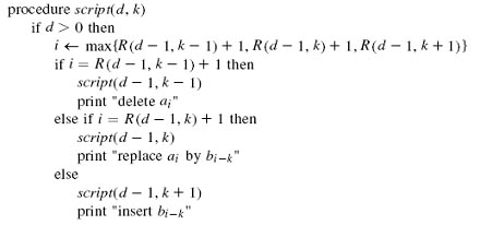
An algorithm to determine an optimal edit script.
A more subtle analysis would show that under certain probabilistic assumptions, the expected running time is O(d2max + L.
BLAST2
'BLAST 2 Sequences', a new BLAST-based tool for aligning two protein or nucleotide sequences, is described. While the standard BLAST program is widely used to search for homologous sequences in nucleotide and protein databases, one often needs to compare only two sequences that are already known to be homologous, coming from related species or, e.g. different isolates of the same virus. In such cases searching the entire database would be unnecessarily time-consuming. 'BLAST 2 Sequences' utilizes the BLAST algorithm for pairwise DNA-DNA or protein-protein sequence comparison. A World Wide Web version of the program can be used interactively at the NCBI WWW site (www.ncbi.nlm.nih.gov/blast/bl2seq/wblast2.cgi). The resulting alignments are presented in both graphical and text form. The variants of the program for PC (Windows), Mac and several UNIX-based platforms can be downloaded from the NCBI FTP site (ftp://ncbi.nlm.nih.gov).
BLAST is a rapid sequence comparison tool that uses a heuristic approach to construct alignments by optimizing a measure of local similarity. Since BLAST compares protein and nucleotide sequences much faster than dynamic programming methods such as Smith-Waterman and Needleman-Wunsch, it is widely used for database searches. A number of important scienti¢c contexts, however, involve the comparison of only two sequences and do not require a time-consuming database search. This happens for example, when one compares a series of viral isolates that may di¡er in only several nucleotide residues per genome. Ongoing projects of sequencing closely related microbial genomes, such as the genomes of Helicobacter pylori strains 26695 and J99, make this a very common task. To meet these needs we have developed a program that uses the BLAST algorithm to produce reliable sequence alignments, without computer-intensive and timeconsuming database searches. The BLAST 2 SEQUENCES program finds multiple local alignments between two sequences, allowing the user to detect homologous protein domains or internal sequence duplications. BLAST 2 SEQUENCES has been very useful for the comparison of homologous genes from complete microbial genomes. Using BLAST 2 SEQUENCES for nucleotide sequence comparison of di¡erent strains or isolates of the same virus o¡ers a convenient strategy to study the genome variations and evolutionary events, such as substitutions, insertions and deletions.
Algorithm
`BLAST 2 SEQUENCES' is an interactive tool that utilizes the BLAST engine for pairwise DNA-DNA or protein-protein sequence comparison and is based on the same algorithm and statistics of local alignments that have been described earlier. The BLAST 2.0 algorithm generates a gapped alignment by using dynamic programming to extend the central pair of aligned residues. The heuristic methods confine the alignments to a prede¢ned region of the path graph. A performance evaluation of the new gapped BLAST algorithm and its comparison to that of the original ungapped BLAST and the Smith-Waterman algorithm have been presented.
The `BLAST 2 SEQUENCES' interface allows the user to perform a series of searches with various parameters. The program can align hundreds of sequences within a reasonable time. Different scoring matrices are provided for protein-protein comparisons; each matrix is most sensitive at finding similarities at a speci¢c evolutionary distance. The default matrix, BLOSUM62 is generally considered to be the best for a wide variety of distances.
Changing the gap existence and extension penalties may change the number and length of gaps in an alignment. There is no analytical formula that determines the `best' gap values to use, so that one may wish to experiment with values in order to explore more of the alignment `space'. BLAST 2.0 uses alone gap costs, which assess a score (a+bk) for a gap of length `k'; long gaps do not cost much more than short ones. Note that only limited values for the gap existence and extension penalties are supported, so that Karlin-Altschul statistics can be applied. The default values of parameters are set up by Javascript function. Selection of the scoring matrix changes the default values of the gap penalties. An incorrect parameter setting returns an error response and brings back the main page, allowing the user to change the selection.
Both protein and nucleotide sequences may contain regions of low compositional complexity, which give spuriously high BLAST scores that re£ect compositional bias rather than signi¢cant position by position alignment. The SEG program can be used for proteins and the DUST program (Tatusov and Lipman, in preparation) for nucleotides if the `Filter' parameter is set. One may also wish to view alignments without a complexity filter, especially if it seems possible that an important part of the aligned sequence has been filtered over. In that case the dot-plot display notes the locations that would have been masked.
BLAST initiates extensions between sequences using a word, meaning that alignments need to share similarity along at least a `word size' number of letters. The default value is 11 for nucleotide-nucleotide alignments and an exact match of `word size' nucleotides between the two sequences is required; three is the default value for protein-protein matches and the sequences may merely be similar along the words, according to the matrix selected. If better sensitivity is needed, one should use a smaller value for the `word size', but it is restricted to the range 7^20 for nucleotide comparisons and 2^3 for proteins. The gapped BLAST 2.0 alignment algorithm uses dynamic programming to extend a central pair of aligned residues in both directions. This approach considers only the alignments that drop in score no more than `x_dropo¡' below the best score yet found. Increasing the `x_dropo¡' value increases the ability to produce a single gapped alignment rather than a collection of ungapped ones. Usually the value of 50 is enough to produce a single gapped alignment for an expected signi¢cance of 10, though these parameters may vary with the scoring system and gap costs. The expectation value is the expected frequency of the matches to be found merely by chance, according to the stochastic model of Karlin and Altschul. To evaluate the statistical significance we choose to use the expectation value over the entire database search rather than the pairwise expectation. That makes it easier to compare the results of pairwise alignment with the results of the data base searches.
The program is not generally useful for motif-style searching and aligning megabase size genomic sequences is not recommended. The maximum number of characters per sequence, that may be accommodated isV150 kb, the optimal size of query sequence is about 1 kb.
The result page starts with the values of parameters that were selected to produce the results. The user can recalculate the alignments by changing the parameters from this page and clicking on the `Align' button, which provides a fast and convenient way of comparing the results for di¡erent values of parameters. It might be useful to compare the results of protein-protein alignments for di¡erent scoring matrices or change the expectation value. The graphical representation shows schematically the set of gapped local alignments found between the two sequences with gaps shown in red. Clicking on the graphics brings the user to the detailed representation of that alignment described below. The dot plot picture provides the user with an overview of sequence similarity. The detailed view for each segment of alignment includes the statistics with the percentage of identities, positives and gaps, schematic view, and the text alignment view. Note that the statistics are calculated based on the size of the NCBI non-redundant database. The bit score reported is the raw score converted to bits of information by multiplying by the Lambda parameter, with the raw score shown in brackets. The expectation value reports shows the number of alignments with that score one expects to ¢nd by chance. If the sequences are taken from the GenBank database and de¢ned by gi or an accession number the hot link to the Entrez query system will be provided. The last part of the report shows the parameters of the calculations and the summary of BLAST statistics. The report is the same as the regular BLAST report, providing an easy way to compare the results of the alignment of two sequences with the results of an entire database search.