Analysis of Protein and Nucleic acid sequences
Protein and Nucleic acid sequences were analyzed by sequence alignment analysis. Different alignment methods like Pair-wise sequence alignment, Multiple sequence alignment, Local alignment and global alignment methods were used. Different scoring matrices like PAM, BLOSUM and PSSM matrices were utilized.
Sequence alignment
Sequence alignment is the process of lining up two or more sequences to achieve maximal levels of identity (and conservation, in the case of amino acid sequences) for the purpose of assessing the degree of similarity and the possibility of homology. Sequence similarity analysis is the single most powerful method for structural and functional inference available in databases. Sequence similarity analysis allows the inference of homology between proteins and homology can help one to infer whether the similarity in sequences would have similarity in function. Methods of analysis can be grouped into two categories– (i) sequence alignment based search, (ii) profile-based search.
Fundamentally, sequence-based alignment searches are string-matching procedures. A sequence of interest (the query sequence) is compared with sequences (targets) in a databank either pair-wise (two at a time) or with multiple target sequences, by searching for a series of individual characters. Two sequences are aligned by writing them across a page in two rows. Identical or similar characters are placed in the same column and non-identical characters can be placed opposite a gap in the other sequence. Gap is a space introduced into an alignment to compensate for insertions and deletions in one sequence relative to another. In optimal alignment, non-identical characters and gaps are placed to bring as many identical or similar characters as possible into vertical register.
The objective of sequence alignment analysis is to analyze sequence data to make reliable prediction on protein structure, function and evolution vis a vis the three-dimensional structure. Such studies include detection of orthologous (same function in different species), and paralogous (different but related functions within an organism) features. Analysis procedures include various statistical algorithms for sequence alignment, pattern matching and prediction of structure directly from sequence. Sequences that are highly divergent during evolution cannot be detected by simple sequence similarity search methods. In such cases, computational methods, comprising multiple sequence alignment and profile-matching searches that go beyond simple pair-wise sequence similarity methods, are tested for meaningful results.
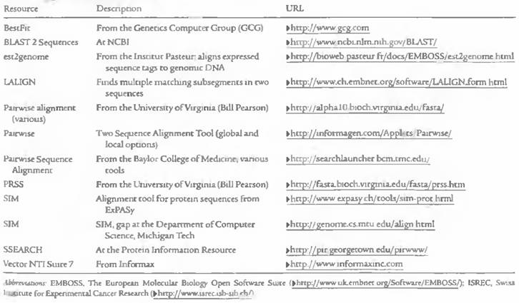
Alignment programs for pair-wise alignment and multiple sequence alignment were listed in the following tables:
Local Pair-wise alignment programs:
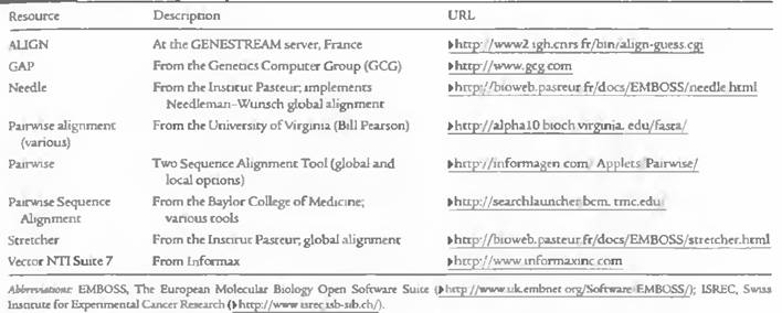
Global Pair-wise alignment Program:
Multiple Sequence alignment programs:
Pairwise sequence alignment:
Pair-wise alignment is a fundamental process in sequence comparison analysis. Pair-wise alignment of two sequences (DNA or protein) is relatively straightforward computational problem. In a pair-wise comparison, if gaps or local alignments are not considered (i.e. fixedlength sequences), the optimal alignment method can be tried and the number of computations required for two sequences is roughly proportional to the square of the average length, as is the case in dotplot comparison. The problem becomes complicated, and not feasible by optimal alignment method, when gaps and local alignments are considered. That a program may align two sequences is not a proof that a relationship exists between them. Statistical values are used to indicate the level of confidence that should be attached to an alignment. A maximum match between two sequences is defined to be the largest number of amino acids from on protein that can be matched with those of another protein, while allowing for all possible deletions. A penalty is introduced to provide a barrier to arbitrary gap insertion.
Sequence Homology and Similarity:
An important concept in sequence analysis is sequence homology. When two sequences are descended from a common evolutionary origin, they are said to have a homologous relationship or share homology. A related but different term is sequence similarity, which is the percentage of aligned residues that are similar in physiochemical properties such as size, charge, and hydrophobicity. It is important to distinguish sequence homology from the related term sequence similarity because the two terms are often confused by some researchers who use them interchangeably in scientific literature. To be clear, sequence homology is an inference or a conclusion about a common ancestral relationship drawn from sequence similarity comparison when the two sequences share a high enough degree of similarity.
On the other hand, similarity is a direct result of observation from the sequence alignment. Sequence similarity can be quantified using percentages; homology is a qualitative statement. For example, one may say that two sequences share 40% similarity. It is incorrect to say that the two sequences share 40% homology. They are either homologous or nonhomologous.
Generally, if the sequence similarity level is high enough, a common evolutionary relationship can be inferred. In dealing with real research problems, the issue of at what similarity level can one infer homologous relationships is not always clear. The answer depends on the type of sequences being examined and sequence lengths. Nucleotide sequences consist of only four characters, and therefore, unrelated sequences have at least a 25% chance of being identical. For protein sequences, there are twenty possible amino acid residues, and so two unrelated sequences can match up 5% of the residues by random chance. If gaps are allowed, the percentage could increase to 10–20%. Sequence length is also a crucial factor. The shorter the sequence, the higher the chance that some alignment is attributable to random chance. The longer the sequence, the less likely the matching at the same level of similarity is attributable to random chance.
This suggests that shorter sequences require higher cutoffs for inferring homologous relationships than longer sequences. For determining a homology relationship of two protein sequences, for example, if both sequences are aligned at full length, which is 100 residues long, an identity of 30% or higher can be safely regarded as having close homology. They are sometimes referred to as being in the “safe zone” (Fig.). If their identity level falls between 20% and 30%, determination of homologous relationships in this range becomes less certain. This is the area often regarded as the “twilight zone,” where remote homologs mix with randomly related sequences.
Below 20% identity, where high proportions of nonrelated sequences are present, homologous relationships cannot be reliably determined and thus fall into the “midnight zone.” It needs to be stressed that the percentage identity values only provide a tentative guidance for homology identification. This is not a precise rule for determining sequence relationships, especially for sequences in the twilight zone.Astatistically more rigorous approach to determine homologous relationships is introduced in the section on the Statistical Significance of Sequence Alignment.
Sequence Similarity and Identity:
Another set of related terms for sequence comparison are sequence similarity and sequence identity. Sequence similarity and sequence identity are synonymous for nucleotide sequences. For protein sequences, however, the two concepts are very different. In a protein sequence alignment, sequence identity refers to the percentage of matches of the same amino acid residues between two aligned sequences. Similarity refers to the percentage of aligned residues that have similar physicochemical characteristics and can be more readily substituted for each other. There are two ways to calculate the sequence similarity/identity. One involves the use of the overall sequence lengths of both sequences; the other normalizes by the size of the shorter sequence. The first method uses the following formula:
S = [(Ls × 2)/(La + Lb)] × 100
where S is the percentage sequence similarity, L s is the number of aligned residues with similar characteristics, and L a and L b are the total lengths of each individual sequence. The sequence identity (I%) can be calculated in a similar fashion:
I = [(Li × 2)/(La + Lb)] × 100
where L i is the number of aligned identical residues. The second method of calculation is to derive the percentage of identical/similar residues over the full length of the smaller sequence using the formula:
I(S)% = Li(s)/La%
where L a is the length of the shorter of the two sequences.
Homology
(a) Similarity attributed to descent from a common ancestor. (NCBI)
(b) Similarity in DNA or protein sequences between individuals of the same species or among different species. (ORNL).
(c) Evolutionary descent from a common ancestor due to gene duplication. (SMART)
Similarity
The extent to which nucleotide or protein sequences are related. The extent of similarity between two sequences can be based on percent sequence identity and/or conservation. In BLAST similarity refers to a positive matrix score. (NCBI)
Identity
The extent to which two (nucleotide or amino acid) sequences are invariant. (NCBI)
Homologues are thus components or characters (such as genes/proteins with similar sequences) that can be attributed to a common ancestor of the two organisms during evolution. Homologues can either be orthologues, paralogues, or xenologues
Orthologues are homologues that have evolved from a common ancestral gene by speciation. They usually have similar functions.
Paralogues are homologues that are related or produced by duplication within a genome. They often have evolved to perform different functions.
Xenologues are homologues that are related by an interspecies (horizontal transfer) of the genetic material for one of the homologues. The functions of the xenologues are quite often similar.
Analogues are non-homologous genes/proteins that have descended convergently from an unrelated ancestor (this is also referred to as 'Homoplasy'). They have similar functions although they are unrelated in either sequence or structure. This is a case of' non-orthologous gene displacement'. In complete contrast to what most researchers instinctively believed, genome comparisons have revealed that this 'nonorthologous gene displacement' occurs at surprisingly high frequency.
Different Methods:
|
S. No |
Method |
Description |
|
1. |
Dot Matrix |
Useful for simple alignments – utilizing graphical methods easy to understand and apply. However it does not show sequences or produce optimal alignment |
|
2. |
Dynamic Programming |
Produces optimal alignment by starting an alignment from one end , then keeping track of all possible best alignments to that point. |
|
3. |
Heuristics Methods |
Fast computational methods. May not be as accurate as dynamic programming. |
Dot Matrix or Dotplot Analysis
Dotplot analysis is essentially a signal-to-noise graph, used in visual comparison of two sequences and to detect regions of close similarity between them (Fig.). The concept of similarity between two sequences can be discerned by dotplots. Two sequences are written along and x- and y-axes, and dots are plotted at all positions where identical residues are observed, that is, at the intersection of every row and column that has the same letter in both the sequences. Within the dotplot, a diagonal unbroken stretch of dots will indicate a region where two sequences are identical. Two similar sequences will be characterized by a broken diagonal; the interrupted region indicating the location of sequence mismatch. A pair of distantly related sequences, with fewer similarities, has a noisier plot (Fig.). Isolated dots that are not on the diagonal represent random matches that are probably not related to any significant alignment. Detection of matching regions may be improved by filtering out random matches in a dotplot. Filtering (overlapping, fixed-length windows etc.) can be used to place a dot only when a group of successive nucleic acid bases (10–15) or amino acid residues (2–3) match, to minimize noise.
Dynamic Programming Method
Dynamic programming is a method for breaking down the alignment of sequences into small parts where one considers all the possible changes in moving from one pair of characters in the alignment to the next. It is comparable to moving across a dot matrix and keeping track of all the matching pairs, adding up those pairs that are along a diagonal and subtracting when insertions are necessary to maintain an alignment. While dot matrix searches provide a great deal of information in a visual fashion, they can only be considered semi-quantitative and therefore do not lend themselves to statistical analysis. Also, dot matrix searches do not provide a precise alignment between two sequences. Dynamic programming, however, can provide global or local alignments.
Global Alignment
Global alignment is an alignment of two nucleic acid or protein sequences over their entire length. The Needleman-Wunsch algorithm (GAP program) is one of the methods to carry out pair-wise global alignment of sequences by comparing a pair of residues at a time. Comparisons are made from the smallest unit of significance, a pair of amino acids, one from each protein. All possible pairs are represented by a two-dimensional array (one sequence along x-axis and the other along y-axis), and pathways through the array represent all possible comparisons (every possible combination of match, mismatch and insertion and deletion). Statistical significance is determined by employing a scoring system; for a match = 1 and mismatch = 0 (or any other relative scores) and penalty for a gap. Each cell in the matrix is examined, maximum score along any path leading to the cell is added to its present contents and the summation is continued. In this way the maximum match (maximum sequence similarity) pathway is constructed. The maximum match is the largest number that would result from summing the cell score values of every pathway, which is defined as the optimal alignment. Leaps to the non-adjacent diagonal cells in the matrix indicate the need for gap insertion, to bring the sequence into register. Complete diagonals of the array contain no gaps.
Needleman-Wunsch algorithm creates a global alignment. That is, it tries to take all the characters of one sequence and align it with all the characters of a second sequence. Needleman-Wunsch algorithm works well for sequences that show similarity across most of their lengths. Globally optimal alignment is a difficult problem (biological sequences may have gaps, insertion sequences relative to each other).
There are limitations to global alignment methods-
1. Global alignment algorithms are often not effective for highly diverged sequences and do not reflect the biological reality that two sequences may only share limited regions of conserved sequence.
2. The influence of global properties for local properties is not valid for all biological sequences.
3. Short and highly similar sub-sequences may be missed in the alignment because the rest of the sequence outweighs them.
Needleman-Wunsch algorithm :
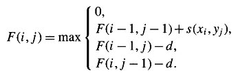
The idea is to build up an optimal alignment using previous solutions for optimal alignments of smaller subsequences. We construct a matrix F indexed by i and j, one index for each sequence, where the value F(i,j) is the score of the best alignment between the initial segment x1..i of x up to xi and the initial segment y1...j of y up to yj. We can build F(i,j) respectively. We begin by initialising F(0,0) = 0. We then proceed to fill the matrix from top left to bottom right. If F(i-1, j-1), F(i-1, j) and F(i, J-1) are known, it is possible to calculate F(i,j). There are three possible ways that the best score F(i,j) of an alignment up to xi, yj could be obtained: xi could be aligned to yj, in which case F(i,j) = F(i-1, j-1) + s(xi,yj) ; or xi is aligned to a gap, in which case F(i,j) = F(i-1, j-1) - d. The best score up to (i,j) will be the largest of these three options. Therefore we have,
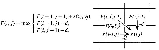
This equation is applied repeatedly to fill in the matrix of F(i,j) values, calculating the value in the bottom right-hand corner of each square of four cells from one of the other three values (above-left, left or above) as in the following figure.
As well fill in the F(i,j) values, we also keep a pointer in each cell back to the cell from which its F(i,j) was derived, as shown in the example of the full dynamic programming matrix. The value in the final cell of the matrix, F(n,m),is by definition the best score for an alignment of x1...n to y1...n, which is what we want; the score of the best global alignment of x to y. To find the alignment itself, we must find the path of choices from the above equation that led to this final value. The procedure for doing this is known as a traceback. It works by building the alignment in reverse, starting from the final cell, and following the pointers that we stored when building the matrix. At each step in the traceback process we move back from the current cell (i,j) to the one of the cells (i-1, j-1), (i-1, j) or (i, j-1) from which the value F(i,j) was derived. At the same time, we add a pair of symbols onto the front of the current alignment: xi and yj if the steop was to (i-1, j-1), xi and the gap character '-' if the step was to (i-1, j), or '-' and yj if the step ws to (i, j-1). At the end we will reach the start of the matrix, i=j=0. An example of this procedure is shown in the following figure:
GAP (http://bioinformatics.iastate.edu/aat/align/align.html) is a web-based pairwise global alignment program. It aligns two sequences without penalizing terminal gaps so similar sequences of unequal lengths can be aligned. To be able to insert long gaps in the alignment, such gaps are treated with a constant penalty. This feature is useful in aligning cDNA to exons in genomic DNA containing the same gene.
Needle tool from EMBOSS (http://emboss.bioinformatics.nl/cgi-bin/emboss/needle) program uses the Needleman-Wunch global alignment algorithm to find the optimum alignment (including gaps) of two sequences when considereing their entire length.
Local Alignment:
Local alignment is an alignment of some portion of two nucleic acid or protein sequences. Smith-Waterman algorithm is a variation of the dynamic programming approach to generate local optimal alignments, best alignment method for sequences for which no evolutionary relatedness is known. The program finds the region or regions of highest similarity between two sequences, thus generating one or more islands of matches or sub-alignments in the aligned sequences. Local alignments are more suitable and meaningful for (i) aligning sequences that are similar along some of their lengths but dissimilar in others, (ii) sequences that differ in length, or (iii) sequences that share conserved regions or domains. A general approach of the procedure is
(i) A negative score / weight is given to mismatches. Therefore, score drops (from initial zero value) as more and more mismatches are added. Hence, the score will rise in a region of high similarity and then fall outside this region.
(ii) When the scoring matrix value becomes negative, that value is set to zero.
(iii) Each pathway begins fresh with zero score.
(iv) The beginining and end of an optimal path may be found anywhere in the matrix, not just the last row or column as is the case with the Needleman-Wunsch method.
(v) The alignements are produced by starting at the highest-scoring positions in the scoring matrix and following a trace path from those positions up to a box that scores zero.
Smith-Waterman algorithm:
The Smith-Waterman algorithm is a member of the class of algorithms that can calculate the best score and local alignment in the order of mn steps, (where 'n' and 'm' are the lengths of the two sequences). These dynamic programming algorithms were first developed for protein sequence comparison by Smith and Waterman, though similar methods were independently devised during the late 1960's and early 1970's for use in the fields of speech processing and computer science. The alogrithm for finding optimal local alignment is closely related to that described in the previous section for global alignments. There are two differences. First, in each cell in the table, an extra possibility is added to the needleman condition, allowing F(i,j) to take the value 0 if all other options have value less than 0:
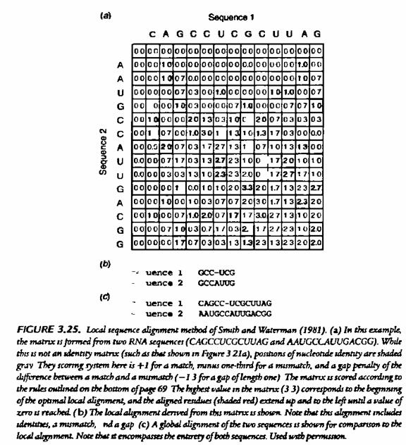
Taking the option 0 corresponds to starting a new alignment. If the best alignment upto some point has a negative score, it is better to start a new one, rather than extend the old one. Note that a consequence of the 0 is that the top row and left column will now be filled with 0s, not -id and -jd as for global alignment. The second change is that now an alignment can end anywhere in the matrix, so instead of taking the value in the bottom right corner, F(n,m), for the best score, we look for the highest value of F(i,j) over the whole matrix and start the traceback from there. The traceback ends when we meet a cell with value 0, which corresponds to the start of the alignment. An example given in the following figure, which shows the best local alignment of the same two sequences whose best global alignment was found in the needle figure. In this case the local alignment is a subset of the global alignment, but that is not always the case.
Water tool from EMBOSS (http://emboss.bioinformatics.nl/cgi-bin/emboss/water) program uses the Smith-Waterman local alignment algorithm.
SIM (http://bioinformatics.iastate.edu/aat/align/align.html) is a web-based program for pairwise alignment using the Smith–Waterman algorithm that finds the best scored nonoverlapping local alignments between two sequences. It is able to handle tens of kilobases of genomic sequence. The user has the option to set a scoring matrix and gap penalty scores. A specified number of best scored alignments are produced.
SSEARCH (http://pir.georgetown.edu/pirwww/search/pairwise.html) is a simple web-based programsthat uses theSmith–Watermanalgorithmfor pairwise alignment of sequences. Only one best scored alignment is given. There is no option for scoring matrices or gap penalty scores.
LALIGN (www.ch.embnet.org/software/LALIGN form.html) is a web-based program that uses a variant of the Smith–Waterman algorithm to align two sequences. Unlike SSEARCH, which returns the single best scored alignment, LALIGN gives a specified number of best scored alignments. The user has the option to set the scoring matrix and gap penalty scores. The same web interface also provides an option for global alignment performed by the ALIGN program.
Heuristic Method
Searching a large database using the dynamic programming methods, such as the Smith–Waterman algorithm, although accurate and reliable, is too slow and impractical when computational resources are limited. An estimate conducted nearly a decade ago had shown that querying a database of 300,000 sequences using a query sequence of 100 residues took 2–3 hours to complete with a regular computer system at the time. Thus, speed of searching became an important issue. To speed up the comparison, heuristic methods have to be used. The heuristic algorithms perform faster searches because they examine only a fraction of the possible alignments examined in regular dynamic programming.
Currently, there are two major heuristic algorithms for performing database searches: BLAST and FASTA. These methods are not guaranteed to find the optimal alignment or true homologs, but are 50–100 times faster than dynamic programming. The increased computational speed comes at a moderate expense of sensitivity and specificity of the search, which is easily tolerated by working molecular biologists. Both programs can provide a reasonably good indication of sequence similarity by identifying similar sequence segments. Both BLAST and FASTA use a heuristic word method for fast pairwise sequence alignment.
BLAST
The BLAST program was developed by Stephen Altschul of NCBI in 1990 and has since become one of the most popular programs for sequence analysis. BLAST uses heuristics to align a query sequence with all sequences in a database. The objective is to find high-scoring ungapped segments among related sequences. The existence of such segments above a given threshold indicates pairwise similarity beyond random chance, which helps to discriminate related sequences from unrelated sequences in a database.
BLAST performs sequence alignment through the following steps. The first step is to create a list of words from the query sequence. Each word is typically three residues for protein sequences and eleven residues for DNA sequences. The list includes every possible word extracted from the query sequence. This step is also called seeding. The second step is to search a sequence database for the occurrence of these words. This step is to identify database sequences containing the matching words. The matching of the words is scored by a given substitution matrix. A word is considered a match if it is above a threshold. The fourth step involves pairwise alignment by extending from the words in both directions while counting the alignment score using the same substitution matrix. The extension continues until the score of the alignment drops below a threshold due to mismatches (the drop threshold is twenty-two for proteins and twenty for DNA). The resulting contiguous aligned segment pair without gaps is called high-scoring segment pair (HSP). In the original version of BLAST, the highest scored HSPs are presented as the final report. They are also called maximum scoring pairs.
The BLAST output includes a graphical overview box, a matching list and a text description of the alignment (Fig). The graphical overview box contains colored horizontal bars that allow quick identification of the number of database hits and the degrees of similarity of the hits. The color coding of the horizontal bars corresponds to the ranking of similarities of the sequence hits (red: most related; green and blue: moderately related; black: unrelated). The length of the bars represents the spans of sequence alignments relative to the query sequence. Each bar is hyperlinked to the actual pairwise alignment in the text portion of the report. Below the graphical box is a list of matching hits ranked by the E-values in ascending order. Each hit includes the accession number, title (usually partial) of the database record, bit score, and E-value. This list is followed by the text description, which may be divided into three sections: the header, statistics, and alignment.
The header section contains the gene index number or the reference number of the database hit plus a one-line description of the database sequence. This is followed by the summary of the statistics of the search output, which includes the bit score, E-value, percentages of identity, similarity (“Positives”), and gaps. In the actual alignment section, the query sequence is on the top of the pair and the database sequence is at the bottom of the pair labeled as Subject. In between the two sequences, matching identical residues are written out at their corresponding positions, whereas nonidentical but similar residues are labeled with “+”. Any residues identified as LCRs in the query sequence are masked with Xs or Ns so that no alignment is represented in those regions.
FASTA
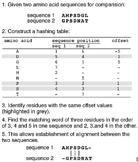
FASTA (FAST ALL, www.ebi.ac.uk/fasta33/) was in fact the first database similarity search tool developed, preceding the development of BLAST. FASTA uses a “hashing” strategy to find matches for a short stretch of identical residues with a length of k. The string of residues is known as ktuples or ktups, which are equivalent to words in BLAST, but are normally shorter than the words. Typically, a ktup is composed of two residues for protein sequences and six residues for DNA sequences. The first step in FASTA alignment is to identify ktups between two sequences by using the hashing strategy. This strategy works by constructing a lookup table that shows the position of each ktup for the two sequences under consideration. The positional difference for each word between the two sequences is obtained by subtracting the position of the first sequence from that of the second sequence and is expressed as the offset. The ktups that have the same offset values are then linked to reveal a contiguous identical sequence region that corresponds to a stretch of diagonal in a two-dimensional matrix (Fig.).
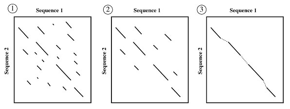
The second step is to narrow down the high similarity regions between the two sequences. Normally, many diagonals between the two sequences can be identified in the hashing step. The top ten regions with the highest density of diagonals are identified as high similarity regions. The diagonals in these regions are scored using a substitution matrix. Neighboring high-scoring segments along the same diagonal are selected and joined to forma single alignment. This step allows introducing gaps between the diagonals while applying gap penalties. The score of the gapped alignment is calculated again. In step 3, the gapped alignment is refined further using the Smith–Waterman algorithm to produce a final alignment (Fig.). The last step is to perform a statistical evaluation of the final alignment as in BLAST, which produces the E-value.
Similar to BLAST, FASTA has a number of subprograms. The web-based FASTA program offered by the European Bioinformatics Institute (www.ebi.ac.uk/) allows the use of either DNA or protein sequences as the query to search against a protein database or nucleotide database. Some available variants of the program are FASTX, which translates aDNAsequence and uses the translated protein sequence to query a protein database, and TFASTX, which compares a protein query sequence to a translated DNA database.
Steps of the FASTA alignment procedure. In step 1 (left ), all possible ungapped alignments are found between two sequences with the hashing method. In step 2 (middle), the alignments are scored according to a particular scoring matrix. Only the ten best alignments are selected. In step 3 (right ), the alignments in the same diagonal are selected and joined to form a single gapped alignment, which is optimized using the dynamic programming approach.
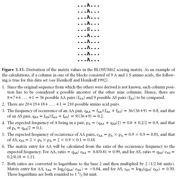
Scoring Matrices
In the dynamic programming algorithm, the alignment procedure has to make use of a scoring system, which is a set of values for quantifying the likelihood of one residue being substituted by another in an alignment. The scoring system is called a substitution matrix and is derived from statistical analysis of residue substitution data from sets of reliable alignments of highly related sequences.
Scoring Matrices for Nucleic Acid Sequences:
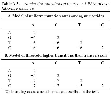
Scoring matrices for nucleotide sequences are relatively simple. A positive value or high score is given for a match and a negative value or low score for a mismatch. This assignment is based on the assumption that the frequencies of mutation are equal for all bases. However, this assumption may not be realistic; observations show that transitions (substitutions between purines and purines or between pyrimidines and pyrimidines) occur more frequently than transversions (substitutions between purines and pyrimidines). Therefore, a more sophisticated statistical model with different probability values to reflect the two types of mutations is needed. A series of nucleic acid PAM matrices based on a Markov transition model similar to that used to generate PAM scoring matrices have been developed.
Scoring Matrices for Amino Acid Sequences
Scoring matrices for amino acids are more complicated because scoring has to reflect the physicochemical properties ofaminoacid residues, aswell as the likelihood of certain residues being substituted among true homologous sequences. Certain amino acids with similar physicochemical properties can be more easily substituted than those without similar characteristics. Substitutions among similar residues are likely to preserve the essential functional and structural features. However, substitutions between residues of different physicochemical properties are more likely to cause disruptions to the structure and function. This type of disruptive substitution is less likely to be selected in evolution because it renders nonfunctional proteins.
Amino acid substitution matrices, which are 20 × 20 matrices, have been devised to reflect the likelihood of residue substitutions. There are essentially two types of amino acid substitution matrices. One type is based on interchangeability of the genetic code or amino acid properties, and the other is derived from empirical studies of amino acid substitutions. Although the two different approaches coincide to a certain extent, the first approach, which is based on the genetic code or the physicochemical features of amino acids, has been shown to be less accurate than the second approach, which is based on surveys of actual amino acid substitutions among related proteins. The most popular two scoring matrices are PAM and BLOSUM matrices. A GONNET matrix is not widely used.
PAM Matrices:
The PAM matrices (also called Dayhoff PAM matrices) were first constructed by Margaret Dayhoff, who compiled alignments of seventy-one groups of very closely related protein sequences. PAM stands for “point accepted mutation” (although “accepted point mutation” or APM may be a more appropriate term, PAM is easier to pronounce). Because of the use of very closely related homologs, the observed mutations were not expected to significantly change the common function of the proteins. Thus, the observed amino acid mutations are considered to be accepted by natural selection.
The PAM matrices were subsequently derived based on the evolutionary divergence between sequences of the same cluster. One PAM unit is defined as 1% of the amino acid positions that have been changed. To construct a PAM1 substitution table, a group of closely related sequences with mutation frequencies corresponding to one PAM unit is chosen. Based on the collected mutational data from this group of sequences, a substitution matrix can be derived.
A PAM unit is defined as 1% amino acid change or one mutation per 100 residues. The increasing PAM numbers correlate with increasing PAM units and thus evolutionary distances of protein sequences (Table). For example, PAM250, which corresponds to 20% amino acid identity, represents 250 mutations per 100 residues. In theory, the number of evolutionary changes approximately corresponds to an expected evolutionary span of 2,500 million years. Thus, the PAM250 matrix is normally used for divergent sequences. Accordingly, PAM matrices with lower serial numbers are more suitable for aligning more closely related sequences. The extrapolated values of the PAM250 amino acid substitution matrix are shown in Figure.

Figure: PAM250 amino acid substitution matrix. Residues are grouped according to physicochemical similarities.
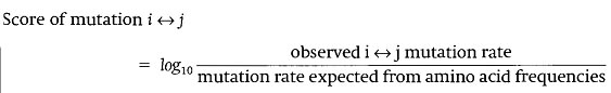
The PAM score for a particular residue pair is derived from a multistep procedure involving calculations of relative mutability (which is the number of mutational changes from a common ancestor for a particular amino acid residue divided by the total number of such residues occurring in an alignment), normalization of the expected residue substitution frequencies by random chance, and logarithmic transformation to the base of 10 of the normalized mutability value divided by the frequency of a particular residue. The resulting value is rounded to the nearest integer and entered into the substitution matrix, which reflects the likelihood of amino acid substitutions. This completes the log-odds score computation. After compiling all substitution probabilities of possible amino acid mutations, a 20 × 20 PAM matrix is established. Positive scores in the matrix denote substitutions occurring more frequently than expected among evolutionarily conserved replacements. Negative scores correspond to substitutions that occur less frequently than expected. Other PAM matrices with increasing numbers for more divergent sequences are extrapolated from PAM1 through matrix multiplication. For example, PAM80 is produced by values of the PAM1 matrix multiplied by itself eighty times.
Steps in the construction of mutation matrix are:
1. Align sequences that are at least 85% identical and determine pair exchange frequencies.
2. Compute frequencies of occurrence.
3. Compute relative mutabilities.
4. Compute a mutation probability matrix.
5. Compute evolutionary distance scale.
6. Calculate log-odds matrix.
1st Step: Pair-exchange frequencies
Aij = Number of times amino acid, j, is replaced by amino acid, i, in all comparisons.
If score = 0; functionally equivalent and/or easily inter-mutable.
If score < 0; two amino acids that are seldom inter-changeable.
2nd Step: Frequencies of occurrence, fi
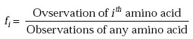
![]()
3rd Step: Relative mutabilities
The amino acids that do not mutate are to be taken into account. This is the relative mutability of the amino acid.
![]()
4th Step: Mutation probability matrix, Mij
![]()
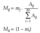
The diagonal elements represent the probability that the amino acid will remain unchanged.
5th Step: The evolutionary distance scale
An evolutionary distance between two sequences is the number of point mutations that was necessary to evolve one sequence into another (the distance is the minimum number of mutations). Since Mii represents the probabilities for amino acids to remain unchanged, multiplying the matrix by l gives the matrix the evolutionary distance of PAM1. The mutation probability is
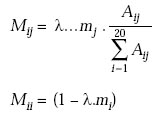
In the framework of this model, a mutation probability matrix for any distance can be obtained by multiplying 1PAM matrix with itself the required number of times.
6th Step: Log-odds matrix
The probability that that some event is observed by random chance pi ran is
![]()
Relatedness

Log-odds matrix, Sij, is the log-odds ratio of two probabilities–probability that two amino acid residues are aligned by evolutionary descendence to the probability that they are aligned by chance.
![]()
S(a,b |t) = log (b|a,t) / qb
Where
P(b|a) = Pab / qa
PAM250 scaled by 3 / log2 to give scores in third bits.
Defects in PAM :
The PAM model is built on the assumptions that are imperfect.
1. The Markov model, that replacement of any site depends only on the amino acid at that site and the probability given by the table, is an imperfect representation of evolution.
Replacement is not equally probable over entire sequence (e.g. local conserved sequences).
2. Each amino acid position is equally mutable is incorrect. Sites vary considerably in their degree of mutability.
3. Many sequences depart from average amino acid composition.
4. Errors in PAM1 are magnified in extrapolation to PAM250.
5. Model is devised using the most mutable positions rather than the most conserved positions, which reflect chemical and structural properties of importance.
6. Distant relationships can only be inferred.
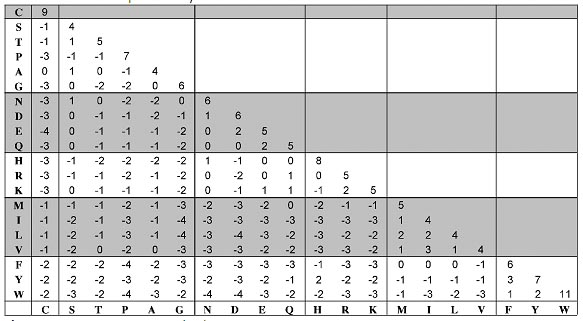
Figure: BLOSUM62 amino acid substitution matrix.
BLOSUM Matrices:
S. Henikoff and J.G. Henikoff developed the family of BLOSUM matrices for scoring substitutions in amino acid sequence comparisons. Their goal was to replace the Dayhoff matrix with one that would perfomr best in identifying distant relationships, making use of the much larger amount of data that had become available since Dayhoff' work. The BLOSUM matrices are based on the BLOCKS databases of aligned protein sequences; hence the name BLOcks SUbstitution Matrix. From regions of closely-related proteins alignable without gaps, Henikoff and Henikoff calculated the ratio of the number of observed pairs of amino acids at any position, to the number of pairs expected from the overall aminoacid frequencies. Like the Dayhoff matrix, the results are expressed as log-adds. In order to avoid overweighting closely-related sequences, the Henikoffs replaced groups of proteins that have sequence identifies higher than a threshold by either a single representative or a weighted average. The threshold 62% produces the commonly-used BLOSUM62 substitution matrix. This is offered by all programs as an option and as the default by most. BLOSUM matrices, and other recently-derived substitution parameters, have superseded the Dayhoff matrix in applications.
The BLOSUM62 matrix is the best for detecting the majority of weak protein similarities and the BLOSUM45 matrix is the best for detecting long and weak alignments. BLOSUM approach can be summarized as follows:
v Locally align each feature to get “blocks”
v Blocks are locally conserved regions, i.e. more constrained regions likely to be related to structure and function
v Blocks contain sequences at all different evolutionary distances and may be highly biased
v Dealing with bias and distance
o Cluster all sequences with less than X% identies
o Clustered sequences count as one sequence
o If X is 100% it simply remove identical sequences
o If X < 100% it reduces the weight on closely related sequences
v Calculate substitution frequencies and log-odds matrix. This give BLOSUMX table.
S(a,b) = log Pab / qa.qb
The log odd values are multiplied by 2 / log2 for BLOSUM62 matrix
The better reliability of blocks method is due to-
1. Many sequences from aligned families are used to generate matrices.
2. Any potential bias introduced by counting multiple contributions from identical residue pairs is removed by clustering sequence segments on the basis of minimum percentage identity.
3. Clusters are treated as single sequences (Blosum60; Blosum80 etc.).
4. Log-odds matrix is calculated from the frequencies, Aij, of observing residue, i, in one cluster aligned against residue, j, in another cluster.
5. Derived from data representing highly conserved sequence segments from divergent proteins rather than data based on very similar sequences (as is the case with PAM matrices).
6. Detects distant similarities more reliably than Dayhoff matrices.
|
S. No |
PAM |
BLOSUM |
|
1. |
Based on explicit evolutionary model |
Based on empirical frequencies |
|
2. |
Represents a specific evolutionary distance |
Always a blend of distances as seen in the database and PROSITE |
|
3. |
Ranges from identical to completely random |
Narrower range than PAM matrix |
|
4. |
Global alignment best result |
Local alignment best result |
Gap Penalties:
Performing optimal alignment between sequences often involves applying gaps that represent insertions and deletions. Because in natural evolutionary processes insertion and deletions are relatively rare in comparison to substitutions, introducing gaps should be made more difficult computationally, reflecting the rarity of insertional and deletional events in evolution. However, assigning penalty values can be more or less arbitrary because there is no evolutionary theory to determine a precise cost for introducing insertions and deletions. If the penalty values are set too low, gaps can become too numerous to allow even nonrelated sequences to be matched up with high similarity scores. If the penalty values are set too high, gaps may become too difficult to appear, and reasonable alignment cannot be achieved, which is also unrealistic. Through empirical studies for globular proteins, a set of penalty values have been developed that appear to suit most alignment purposes. They are normally implemented as default values in most alignment programs.
Another factor to consider is the cost difference between opening a gap and extending an existing gap. It is known that it is easier to extend a gap that has already been started. Thus, gap opening should have a much higher penalty than gap extension. This is based on the rationale that if insertions and deletions ever occur, several adjacent residues are likely to have been inserted or deleted together. These differential gap penalties are also referred to as affine gap penalties. The normal strategy is to use preset gap penalty values for introducing and extending gaps. For example, one may use a −12/ − 1 scheme in which the gap opening penalty is −12 and the gap extension penalty −1.
Affine gap penalty is a type of gap penalty that penalizes insertions and deletions using a linear function in which one term is length independent and the other is length dependent. A regular gap extension method would assign a fixed cost per gap. An affine gap penalty encourages the extension of gaps rather than the introduction of new gaps. The total gap penalty (W) [affine gap score] is a linear function of gap length, which is calculated using the formula:
W = γ + δ (k− 1)
where γ is the gap opening penalty, δ is the gap extension penalty, and k is the length of the gap. Besides the affine gap penalty, a constant gap penalty is sometimes also used, which assigns the same score for each gap position regardless whether it is opening or extending. However, this penalty scheme has been found to be less realistic than the affine penalty.
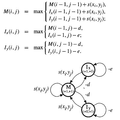
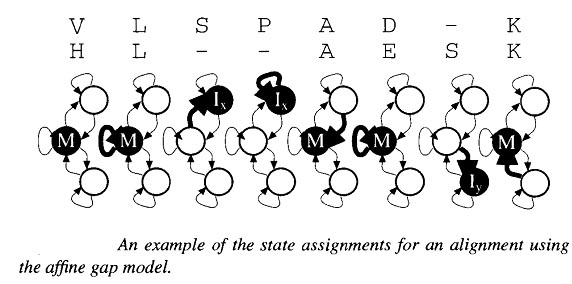
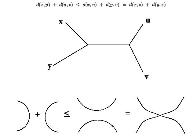
The system defined by the above equations can be described very elegently by the above diagrm. This shows a state for each of the three matrix values, with transition arrows between states. The transitions each carrry a score increment , and the states each specify a D(i,j) pair, which is used to determine the change in indices i and j when that state is entered. The recurrence relation for updating each matrix value can be read directly from the diagram. The new value for a state variable at (i,j) is the maximum of the scores corresponding to the transitions coming to the state. Each transition score is given by the value of the source state at the offsets specified by the D(i,j) pair of the target state, plus the specified score increment. This type of description corresponds to a finite state automation (FSA) in computer science. An alignemtn corresponds to a path through the states, with symbols from the underlying pair of sequences being transferred to the alignment accoring to the D(i,j) values in the states. An example of a short alignment and corresponding state path through the affine gap model in the following figure. It is in fact frequent practice to implement an affine gap cost algorithm using only to states, M and I where I represents the possiblity of being in a gapped regions.
Difference between Distance and Similarity matrix:
Trees that represent protein or nucleic acid sequences usually display the differences between various sequences. One way to measure distances is to count the number of mismatches in a pairwise alignment. Another method, employed by the Feng and Doolittle progressive alignment algorithm, is to convert similarity scores to distance scores. Similarity scores are calculated from a series of pairwise alignments among all the proteins being multiply aligned. The similarity scores S between two sequences (i, j) are converted to distance scores D using the equation
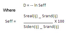
Here, Sreal(ij ) describes the observed similarity score for two aligned sequences i and j, Siden(ij ) is the average of the two scores for the two sequences compared to themselves (if score i compared to i receives a score of 20 and score j compared to j receives a score of 10, then Siden(ij ) =15); Srand(ij ) is the mean alignment score derived from many (e.g., 1000) random shufflings of the sequences; and Seff is a normalized score. If sequences i, j have no similarity, then Seff = 0 and the distance is infinite. If sequences i, j are identical, then Seff = 1 and the distance is 0.
Similarity matrices are used for database searching, while distance matrices are naturally used for phylogenetic tree construction. The distance score (D) is usually calculated by summing up of mismatches in an alignment divided by the total number of matches and mismatches, which represents the number of changes required to change one sequence into the other, ignoring gaps.
Matches
D = --------------------------------------------
(Matches + Mismatches)
By determining the number of mutational changes by sequence alignment methods, a quantitative measure can be obtained of the distance between any pair of sequences. These values can be used to reconstruct a phylogenetic tree, which describes a relationship between the gene sequences. The more mutations required changing one sequence into the other, the more unrelated the sequences and the lower the probability that they share a recent common ancestor sequence. Conversely, the more alike a pair of sequences, the fewer the number of changes required to change one sequence into the other, and the greater the likelihood that they share a recent common ancestor sequence.
Distances between DNA sequences are relatively simple to compute as the sum between two sequences, that is the least number of steps required to change one sequence into the other (D = X + Y). It is preferable in phylogenetic tree analysis because (i) the pattern of mutations, insertions and deletions at the nucleotide level are definitive and (ii) silent mutations at the DNA level do not result in an amino acid substitution (because of the redundancy of the genetic code). A simple matrix of the frequencies of the 12 possible types of replacement (each base can be replaced by any of the three other bases) can be used. Differences due to insertions/deletions are generally given a large score than substations.
Simple similarity matrix for DNA:
The simplest matrix in use is the identity (similarity) matrix. If two letters are the same they are given +1 and 0 if they are not the same.
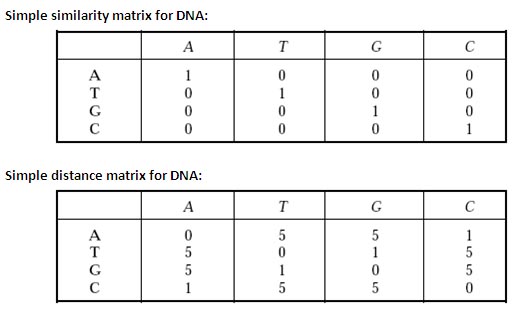
Simple distance matrix for DNA:
Nucleotide bases fall into two classes depending on the ring structure of bases— two-ring purine bases (A and G) and single-ring pyrimidine bases (T and C). A mutation that conserves the ring number (A « G; or T « C) is called transition and a mutation that changes the ring number (purine « pyrimidine) is called transversion. Use of transition/transversion matrix with weighted scores reduces noise in comparisons of distantly related sequences.
Distances between amino acid sequences are more difficult to calculate, because
1. Some amino acids can be changed due to replacement of single DNA base (single-point mutation), while replacement of other amino acids require two or three base changes within the DNA sequence.
2. While conservative mutations of amino acids do not have much effect on the structure and function, other replacements can be functionally lethal.
Since all point mutations arise from nucleotide changes, the probability that an observed amino acid pair is related by chance, rather than by inheritance should depend only on the number of point mutations necessary to transform one codon into the other. A matrix resulting from this model would define the distance between two amino acids by the minimal number of the nucleotide changes required (genetic code matrix). It may be more useful to compare the sequences of the purine (R)-pyrimidine level. To this can be added other physicochemical attributes of amino acids (hydrophobicity matrix, size and volume matrix etc.).
Assessing the significance of sequence alignment:
One of the most important recent advances in sequence analysis is the development of methods to assess the significance of an alignment between DNA or protein sequences. For sequences that are quite similar, such as two proteins that are clearly in the same family, such an analysis is not necessary. A significance question arises when comparing two sequences that are not so clearly similar but are shown to align in the promising way. In such a case, a significance test can help the biologist to decide whether an alignment found by the computer program is one that would be expected between related sequences or would just as likely be found if the sequences were not related. The significance test is also needed to evaluate the results of a database search for sequences that are similar to a sequence by the BLAST and FASTA programs. The test will be applied to every sequence matched so that the most significant matches are reported. Finally, a significance test can also help to identify regions in a single sequence that have an unusual composition suggestive of an interesting function. Our present purpose is to examine the significance of sequence alignment scores obtained by the dynamic programming method.
Significance of Local Alignment:
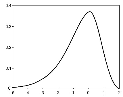
Solving this problem requires a statistical test of the alignment scores of two unrelated sequences of the same length. By calculating alignment scores of a large number of unrelated sequence pairs, a distribution model of the randomized sequence scores can be derived. From the distribution, a statistical test can be performed based on the number of standard deviations from the average score. Many studies have demonstrated that the distribution of similarity scores assumes a peculiar shape that resembles a highly skewed normal distribution with a long tail on one side (Fig.). The distribution matches the “Gumble extreme value distribution” for which a mathematical expression is available. This means that, given a sequence similarity value, by using the mathematical formula for the extreme distribution, the statistical significance can be accurately estimated.
The statistical test for the relatedness of two sequences can be performed using the following procedure. An optimal alignment between two given sequences is first obtained. Unrelated sequences of the same length are then generated through a randomization process in which one of the two sequences is randomly shuffled. A new alignment score is then computed for the shuffled sequence pair. More such scores are similarly obtained through repeated shuffling. The pool of alignment scores from the shuffled sequences is used to generate parameters for the extreme distribution. The original alignment score is then compared against the distribution of random alignments to determine whether the score is beyond random chance. If the score is located in the extreme margin of the distribution, that means that the alignment between the two sequences is unlikely due to random chance and is thus considered significant. A P-value is given to indicate the probability that the original alignment is due to random chance.
A P-value resulting from the test provides a much more reliable indicator of possible homologous relationships than using percent identity values. It is thus important to know how to interpret the P-values. It has been shown that if a P-value is smaller than 10−100, it indicates an exact match between the two sequences. If the P-value is in the range of 10−50 to 10−100, it is considered to be a nearly identical match. A P-value in the range of 10−5 to 10−50 is interpreted as sequences having clear homology. A P-value in the range of 10−1 to 10−5 indicates possible distant homologs. If P is larger than 10−1, the two sequence may be randomly related. However, the caveat is that sometimes truly related protein sequences may lack the statistical significance at the sequence level owing to fast divergence rates. Their evolutionary relationships can nonetheless be revealed at the three-dimensional structural level.
These statistics were derived from ungapped local sequence alignments. It is not known whether the Gumble distribution applies equally well to gapped alignments. However, for all practical purposes, it is reasonable to assume that scores for gapped alignments essentially fit the same distribution. A frequently used software program for assessing statistical significance of a pairwise alignment is the PRSS program. PRSS (Probability of Random Shuffles; www.ch.embnet.org/software/PRSS form.html) is a web-based program that can be used to evaluate the statistical significance of DNA or protein sequence alignment. It first aligns two sequences using the Smith–Waterman algorithm and calculates the score. It then holds one sequence in its original form and randomizes the order of residues in the other sequence. The shuffled sequence is realigned with the unshuffled sequence. The resulting alignment score is recorded. This process is iterated many (normally 1,000) times to help generate data for fitting the Gumble distribution. The original alignment score is then compared against the overall score distribution to derive a P-value. The major feature of the program is that it allows partial shuffling. For example, shuffling can be restricted to residues within a local window of 25–40, whereas the residues outside the window remain unchanged.
Significance of global alignment:
In general, global alignment program use the Needleman-Wunsch alignment algorithm and a scoring system that scores the average match of an aligned nucleotide or amino acid pair as a positive number. Hence, the score of the alignment of random or unrelated sequences grows proportionally to the length of the sequences. In addition, there are many possible different global alignments depending on the scoring system chosen and small changes in the scoring system can produce a different alignment. Thus, finding the best global alignment and knowing how to assess its significance is not a simple task, as reflected by the absence of studies in the literature. The GCG alignment programs have a RANDOMIZATION option, which shuffles the second sequence and calculates similarity scores between the unshuffled sequence and each of the shuffled copies. If the new similarity scores are significantly smaller than the real alignment score, the alignment is considered significant. This analysis is only useful for providing a rough approximation of the significance of an alignment score and can easily be misleading.
Dayhoff (1978) and Dayhoff et al. (1983) devised a second method for testing the relatedness of two protein sequnences that can accommodate some local variation. This method is useful for finding repeated regions within a sequence, similar regions that are in a different order in two sequences, or a small conserved region such as an active site. As used in a computer program called RELATE, all possible segments of a given length of one sequence are compared with all segments of the same length from another. An alignment score using a scoring matrix is obtained for each comparison to give a score distribution among all of the segments. A segment comparison score in standard deviation units is calculated as the difference between the value for real sequences minus the average value for random sequences divided by the standard deviation of the scores from the random sequences. A version of the program RELATE that runs on many computer platforms is included with the FASTA distribution package by W.Pearson.
Strings and Evolutionary trees
The dominant view of the evolution of life is that all existing organisms are derived from some common ancestor and that a new species arises by a splitting of one population into two (or more) populations that do not cross-breed, rather than by a mixing of two populations into one. Therefore, the high level history of life is ideally organized and displayed as a rooted, directed tree. The extant species (and some of the extinct species) are represented at the leaves of the tree, each internal node represents a point when the history of two sets of species diverged (or represents a common ancestor of those species), the length and direction of each edge represents the passage of time or the evolutionary events that occur in that time, and so the path from the root of the tree to each leaf represents the evolutionary history of the organisms represented there. Increasingly, the methods to create evolutionary trees are encoded into computer programs and the data used by these programs are based, directly or indirectly, on molecular sequence data. In this chapter we discuss some of the mathematical and algorithmic issues involved in evolutionary tree construction and the interrelationship of tree construction methods to algorithms that operate on strings and sequences.
Additive and Ultrametric Trees
Evolutionary
relationships can be represented by a variety of trees such as the
the Cladogram, Additive, and the Ultrametric Trees.
Cladogram A cladogram is a tree that only represents a branching pattern. The edge lengths do not represent anything.
Phylogram A phylogram is a phylogenetic tree where edge lengths represent time or genetic distance.
Ultrametric tree An ultrametric tree or chronogram is a phylogenetic tree where edge lengths represent time (so current taxa are equidistant from the root).
Additive Tree:
An additive tree is one where along with the topology of the tree edge lengths are also specified corresponding to distances among the organisms. An ultrametric tree is a special kind of a rooted additive tree where the terminal nodes are all equally distant from the root. Additive trees contain additional information, namely branch lengths. These are numbers associated with each branch that corresponds to some attribute of the sequence such as amount of evolutionary change.
An additive tree also is characterized by the four point condition: Any 4 points can be renamed such that
The following algorithm for the reconstruction of an additive tree from a given distance matrix was introduced by Beyer, Singh, Smith and Waterman:
1. The new path branches off an existing branch in the tree: Do the insertion step once more in the branching path.
2. The new path branches off an edge in the tree: This insertion is finished.
An alternative algorithm inserts a new object into the tree by trying to solve the linear equations which result from trying to let the new edge branch off each edge in the tree, whereat there exists a solution for one edge only:
Given a distance matrix constituting an additive metric, the topology of the corresponding additive tree is unique. An additive tree for an additive matrix can be constructed in O(n2) time. The lengths of the branches are showing the distance of each descendents from the ancestor, which is known as additive distance.
Ultrametric tree:
Ultrametric trees are a special kind of additive tree in which the tips of the trees are all equidistant from the root of the tree. This type of tree can be used to express evolutionary time, stated in years or indirectly as the amount of sequence divergence using a molecular clock. An ultrametric tree also is characterized by the three point condition (P. Bunemann): Any three points x, y, z can be renamed such that
![]()
Given a set of sequences and assuming that the pairwise sequence alignments provide a measure for the evolutionary distance between the sequences and that the the resulting distance matrix constitutes an ultrameric (the ideal case), the reconstruction of the phylogenetic, ultrametric tree is managed by the following general clustering procedure:
Always pick the closest pair from the distance matrix and merge these two objects into one. Various schemes differ in how the distance between a newly formed object and the other objects is defined. Say, object x has been formed by merging y and z.
For non-ultrametric distances clustering will produce an ultrametic tree, whose distances will somehow resemble the original matrix. The following figure gives an example for the construction of an ultrametric tree by average linkage clustering. Given is a n x n distance matrix constituting an ultrametric:
A symmetric matrix D of real numbers defines an ultrametric distance if and only if for every three indices/, j , and k, there is a tie for the maximum of D(i, j), D(i, k), and D(j, k). That is, the maximum of those three numbers is not unique. When D defines an ultrametric distance, we will often say that D is an ultrametric matrix. If D is an ultrametric matrix, then an ultrametric tree for D can be constructed in O(n2) time.
PHYLOGENETICS
In biology, phylogenetics is the study of evolutionary relatedness among groups of organisms (e.g. species, populations), which is discovered through molecular sequencing data and morphological data matrices. The term phylogenetics derives from the Greek terms phyle and phylon, denoting “tribe” and “race”; and the term genetikos, denoting “relative to birth”, from genesis “birth”.
Taxonomy, the classification, identification, and naming of organisms, is richly informed by phylogenetics, but remains methodologically and logically distinct. The fields of phylogenetics and taxonomy overlap in the science of phylogenetic systematics — one methodology, cladism (also cladistics) shared derived characters (synapomorphies) used to create ancestor-descendant trees (cladograms) and delimit taxa (clades). In biological systematics as a whole, phylogenetic analyses have become essential in researching the evolutionary tree of life.
phylogenetic tree
A phylogenetic tree or evolutionary tree is a branching diagram or "tree" showing the inferred evolutionary relationships among various biological species or other entities based upon similarities and differences in their physical and/or genetic characteristics. The taxa joined together in the tree are implied to have descended from a common ancestor. In a rooted phylogenetic tree, each node with descendants represents the inferred most recent common ancestor of the descendants, and the edge lengths in some trees may be interpreted as time estimates. Each node is called a taxonomic unit. Internal nodes are generally called hypothetical taxonomic units (HTUs) as they cannot be directly observed. Trees are useful in fields of biology such as bioinformatics,systematics and comparative phylogenetics.
A rooted phylogenetic tree is a directed tree with a unique node corresponding to the (usually imputed) most recent common ancestor of all the entities at the leaves of the tree. The most common method for rooting trees is the use of an uncontroversial outgroup — close enough to allow inference from sequence or trait data, but far enough to be a clear outgroup.
Unrooted trees illustrate the relatedness of the leaf nodes without making assumptions about ancestry at all. While unrooted trees can always be generated from rooted ones by simply omitting the root, a root cannot be inferred from an unrooted tree without some means of identifying ancestry; this is normally done by including an outgroup in the input data or introducing additional assumptions about the relative rates of evolution on each branch, such as an application of the molecular clock hypothesis. Figure 1 depicts an unrooted phylogenetic tree for myosin, a superfamily of proteins.
A dendrogram is a broad term for the diagrammatic representation of a phylogenetic tree.
A cladogram is a phylogenetic tree formed using cladistic methods. This type of tree only represents a branching pattern, i.e., its branch lengths do not represent time or relative amount of character change.
A phylogram is a phylogenetic tree that has branch lengths proportional to the amount of character change.
A chronogram is a phylogenetic tree that explicitly represents evolutionary time through its branch lengths.
Computational phylogenetics
Computational phylogenetics is the application of computational algorithms, methods and programs to phylogenetic analyses. The goal is to assemble a phylogenetic tree representing a hypothesis about the evolutionary ancestry of a set of genes, species, or other taxa. For example, these techniques have been used to explore the family tree of hominid species and the relationships between specific genes shared by many types of organisms. Traditional phylogenetics relies on morphological data obtained by measuring and quantifying the phenotypic properties of representative organisms, while the more recent field of molecular phylogenetics uses nucleotide sequences encoding genes or amino acid sequences encoding proteins as the basis for classification. Many forms of molecular phylogenetics are closely related to and make extensive use of sequence alignment in constructing and refining phylogenetic trees, which are used to classify the evolutionary relationships between homologous genes represented in the genomes of divergent species. The phylogenetic trees constructed by computational methods are unlikely to perfectly reproduce the evolutionary tree that represents the historical relationships between the species being analyzed. The historical species tree may also differ from the historical tree of an individual homologous gene shared by those species.
Distance-matrix methods
Distance-matrix methods of phylogenetic analysis explicitly rely on a measure of "genetic distance" between the sequences being classified, and therefore they require an MSA as an input. Distance is often defined as the fraction of mismatches at aligned positions, with gaps either ignored or counted as mismatches. Distance methods attempt to construct an all-to-all matrix from the sequence query set describing the distance between each sequence pair. From this is constructed a phylogenetic tree that places closely related sequences under the same interior node and whose branch lengths closely reproduce the observed distances between sequences. Distance-matrix methods may produce either rooted or unrooted trees, depending on the algorithm used to calculate them. They are frequently used as the basis for progressive and iterative types of multiple sequence alignments. The main disadvantage of distance-matrix methods is their inability to efficiently use information about local high-variation regions that appear across multiple subtrees.
UPGMA
In Figure, the UPGMA method is applied to the data sample. At each cycle of the method, the smallest entry is located, and the entries intersecting at that cell are "joined." The height of the branch for this junction is one-half the value of the smallest entry. Thus, since the smallest entry at the beginning is 1 (between B=man and F=monkey), B and F are joined with branch heights of 0.5 (=1.0/2). Then, the comparison matrix is reduced by combining cells. These combinations are indicated with colors in Figure 2. For example, the comparisons of A to B (19.0) and A to F (18.0) are consolidated as 18.5 = (19.0+18.0)/2 (red cells), while the comparisons of E to B (36.0) and E to F (35.0.0) are consolidated as 35.5 = (36.0+35.0)/2 (blue cells).
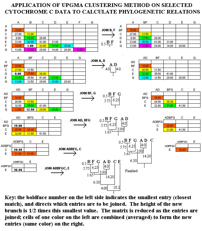
Construction of a distance tree using clustering with the Unweighted Pair Group Method with Arithmatic Mean (UPGMA).
The UPGMA is the simplest method of tree construction. It was originally developed for constructing taxonomic phenograms, i.e. trees that reflect the phenotypic similarities between OTUs, but it can also be used to construct phylogenetic trees if the rates of evolution are approximately constant among the different lineages. For this purpose the number of observed nucleotide or amino-acid substitutions can be used. UPGMA employs a sequential clustering algorithm, in which local topological relationships are identifeid in order of similarity, and the phylogenetic tree is build in a stepwise manner. We first identify from among all the OTUs the two OTUs that are most similar to each other and then treat these as a new single OTU. Such a OTU is referred to as a composite OTU. Subsequently from among the new group of OTUs we identify the pair with the highest similarity, and so on, until we are left with only two UTUs.
The pairwise evolutionary distances are given by the following distance matrix:
|
|
A |
B |
C |
D |
E |
|
B |
2 |
|
|||
|
C |
4 |
4 |
|
||
|
D |
6 |
6 |
6 |
|
|
|
E |
6 |
6 |
6 |
4 |
|
|
F |
8 |
8 |
8 |
8 |
8 |
We now cluster the pair of OTUs with the smallest distance, being A and B, that are separated a distance of 2. The branching point is positioned at a distance of 2 / 2 = 1 substitution. We thus constuct a subtree as follows:

Following the first clustering A and B are considered as a single composite OTU(A,B) and we now calculate the new distance matrix as follows:
dist(A,B),C = (distAC + distBC) / 2 = 4
dist(A,B),D = (distAD + distBD) / 2 = 6
dist(A,B),E = (distAE + distBE) / 2 = 6
dist(A,B),F = (distAF + distBF) / 2 = 8
In other words the distance between a simple OTU and a composite OTU is the average of the distances between the simple OTU and the constituent simple OTUs of the composite OTU. Then a new distance matrix is recalculated using the newly calculated distances and the whole cycle is being repeated:
|
|
A,B |
C |
D |
E |
|
C |
4 |
|
||
|
D |
6 |
6 |
|
|
|
E |
6 |
6 |
4 |
|
|
F |
8 |
8 |
8 |
8 |
|
|
A,B |
C |
D,E |
|
C |
4 |
|
|
|
D,E |
6 |
6 |
|
|
F |
8 |
8 |
8 |
Fourth cycle
|
|
AB,C |
D,E |
|
D,E |
6 |
|
|
F |
8 |
8 |
Fifth cycle
The final step consists of clustering the last OTU, F, with the composite OTU.
|
|
ABC,DE |
|
F |
8 |
Although this method leads essentially to an unrooted tree, UPGMA assumes equal rates of mutation along all the branches, as the model of evolution used. The theoretical root, therefore, must be equidistant from all OTUs. We can here thus apply the method of mid-point rooting. The root of the entire tree is then positioned at dist (ABCDE),F / 2 = 4.
The final tree as inferred by using the UPGMA method is shown below.
So now we have reconstructed the phylogenetic tree using the UPGMA method. As you can see we have obtained the original phylogenetic tree we started with.
Neighbor-joining methods apply general data clustering techniques to sequence analysis using genetic distance as a clustering metric. The simple neighbor-joining method produces unrooted trees, but it does not assume a constant rate of evolution (i.e., a molecular clock) across lineages. Its relative, UPGMA (Unweighted Pair Group Method with Arithmetic mean) produces rooted trees and requires a constant-rate assumption - that is, it assumes an ultrametric tree in which the distances from the root to every branch tip are equal.
The Fitch-Margoliash method uses a weighted least squares method for clustering based on genetic distance. Closely related sequences are given more weight in the tree construction process to correct for the increased inaccuracy in measuring distances between distantly related sequences. The distances used as input to the algorithm must be normalized to prevent large artifacts in computing relationships between closely related and distantly related groups. The distances calculated by this method must be linear; the linearity criterion for distances requires that the expected values of the branch lengths for two individual branches must equal the expected value of the sum of the two branch distances - a property that applies to biological sequences only when they have been corrected for the possibility of back mutations at individual sites. This correction is done through the use of a substitution matrix such as that derived from the Jukes-Cantor model of DNA evolution. The distance correction is only necessary in practice when the evolution rates differ among branches.
The least-squares criterion applied to these distances is more accurate but less efficient than the neighbor-joining methods. An additional improvement that corrects for correlations between distances that arise from many closely related sequences in the data set can also be applied at increased computational cost. Finding the optimal least-squares tree with any correction factor is NP-complete, so heuristic search methods like those used in maximum-parsimony analysis are applied to the search through tree space.
Character Based Methods
Maximum parsimony
Maximum parsimony (MP) is a method of identifying the potential phylogenetic tree that requires the smallest total number of evolutionary events to explain the observed sequence data. Some ways of scoring trees also include a "cost" associated with particular types of evolutionary events and attempt to locate the tree with the smallest total cost. This is a useful approach in cases where not every possible type of event is equally likely - for example, when particular nucleotides or amino acids are known to be more mutable than others.
The most naive way of identifying the most parsimonious tree is simple enumeration - considering each possible tree in succession and searching for the tree with the smallest score. However, this is only possible for a relatively small number of sequences or species because the problem of identifying the most parsimonious tree is known to be NP-hard; consequently a number of heuristic search methods for optimization have been developed to locate a highly parsimonious tree, if not the most optimal in the set. Most such methods involve a steepest descent-style minimization mechanism operating on a tree rearrangement criterion.
Maximum likelihood
The maximum likelihood method uses standard statistical techniques for inferring probability distributions to assign probabilities to particular possible phylogenetic trees. The method requires a substitution model to assess the probability of particular mutations; roughly, a tree that requires more mutations at interior nodes to explain the observed phylogeny will be assessed as having a lower probability. This is broadly similar to the maximum-parsimony method, but maximum likelihood allows additional statistical flexibility by permitting varying rates of evolution across both lineages and sites. In fact, the method requires that evolution at different sites and along different lineages must be statistically independent. Maximum likelihood is thus well suited to the analysis of distantly related sequences, but because it formally requires search of all possible combinations of tree topology and branch length, it is computationally expensive to perform on more than a few sequences.
The "pruning" algorithm, a variant of dynamic programming, is often used to reduce the search space by efficiently calculating the likelihood of subtrees. The method calculates the likelihood for each site in a "linear" manner, starting at a node whose only descendants are leaves (that is, the tips of the tree) and working backwards toward the "bottom" node in nested sets. However, the trees produced by the method are only rooted if the substitution model is irreversible, which is not generally true of biological systems. The search for the maximum-likelihood tree also includes a branch length optimization component that is difficult to improve upon algorithmically; general global optimization tools such as the Newton-Raphson method are often used. Searching tree topologies defined by likelihood has not been shown to be NP-complete, but remains extremely challenging because branch-and-bound search is not yet effective for trees represented in this way.
Cladogram
A cladogram is a diagram used in cladistics which shows ancestral relations between organisms, to represent the evolutionary tree of life. Although traditionally such cladograms were generated largely on the basis of morphological characters, DNA and RNA sequencing data and computational phylogenetics are now very commonly used in the generation of cladograms.
Generating a cladogram
A greatly simplified procedure for generating a cladogram is:
A cladistic analysis begins with the following data:
For example, if analyzing 20 species of birds, the data might be:
All the data are then organized into a "taxon-character matrix", which is the base to perform phylogenetic analysis.
The characteristics used to create a cladogram can be roughly categorized as either morphological (synapsid skull, warm blooded, notochord, unicellular, etc.) or molecular (DNA, RNA, or other genetic information). Prior to the advent of DNA sequencing, all cladistic analysis used morphological data. As DNA sequencing has become cheaper and easier, molecular systematics has become a more and more popular way to reconstruct phylogenies. Using a parsimony criterion is only one of several methods to infer a phylogeny from molecular data; maximum likelihood and Bayesian inference, which incorporate explicit models of sequence evolution, are non-Hennigian ways to evaluate sequence data. Another powerful method of reconstructing phylogenies is the use of genomic retrotransposon markers, which are thought to be less prone to the problem of reversion that plagues sequence data. They are also generally assumed to have a low incidence of homoplasies because it was once thought that their integration into the genome was entirely random; this seems at least sometimes not to be the case, however. Ideally, morphological, molecular, and possibly other phylogenies should be combined into an analysis of total evidence: All have different intrinsic sources of error. For example, character convergence (homoplasy) is much more common in morphological data than in molecular sequence data, but character reversions that are unrecognizable as such are more common in the latter. Morphological homoplasies can usually be recognized as such if character states are defined with enough attention to detail.
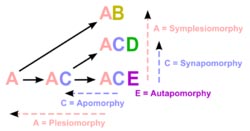
Apomorphy in cladistics
The researcher must decide which character states were present before the last common ancestor of the species group (plesiomorphies) and which were present in the last common ancestor (synapomorphies) and does so by comparison to one or more outgroups. The choice of an outgroup is a crucial step in cladistic analysis because different outgroups can produce trees with profoundly different topologies. Note that only synapomorphies are of use in characterizing clades.
A homoplasy is a character that is shared by multiple species due to some cause other than common ancestry. The two main types of homoplasy are convergence (appearance of the same character in at least two distinct lineages) and reversion (the return to an ancestral character). Use of homoplasies when building a cladogram is sometimes unavoidable but is to be avoided when possible.
A well known example of homoplasy due to convergent evolution would be the character, "presence of wings". Though the wings of birds, bats, and insects serve the same function, each evolved independently, as can be seen by their anatomy. If a bird, bat, and a winged insect were scored for the character, "presence of wings", a homoplasy would be introduced into the dataset, and this would confound the analysis, possibly resulting in a false evolutionary scenario.
Homoplasies can often be avoided outright in morphological datasets by defining characters more precisely and increasing their number. When analyzing "supertrees" (datasets incorporating as many taxa of a suspected clade as possible), it may become unavoidable to introduce character definitions that are imprecise, as otherwise the characters might not apply at all to a large number of taxa; to continue with the "wings" example, the presence of wings would hardly be a useful character if attempting a phylogeny of all Metazoa, as most of these don't have wings at all. Cautious choice and definition of characters thus is another important element in cladistic analyses. With a faulty outgroup or character set, no method of evaluation is likely to produce a phylogeny representing the evolutionary reality.
When there are just a few species being organized, it is possible to do this step manually, but most cases require a computer program. There are scores of computer programs available to support cladistics. Because the total number of possible cladograms grows factorially with the number of species, it is impractical for a computer program to evaluate every individual cladogram. A typical cladistic program begins by using heuristic techniques to identify a small number of candidate cladograms. Many cladistic programs then continue the search with the following repetitive steps:
Computer programs that generate cladograms use algorithms that are very computationally intensive, because the cladogram problem is NP-hard.
There are several algorithms available to identify the "best" cladogram. Most algorithms use a metric to measure how consistent a candidate cladogram is with the data. Most cladogram algorithms use the mathematical techniques of optimization and minimization.
In general, cladogram generation algorithms must be implemented as computer programs, although some algorithms can be performed manually when the data sets are trivial (for example, just a few species and a couple of characteristics).
Some algorithms are useful only when the characteristic data are molecular (DNA, RNA); other algorithms are useful only when the characteristic data are morphological. Other algorithms can be used when the characteristic data includes both molecular and morphological data.
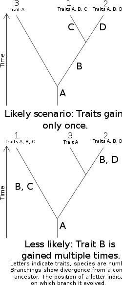
Simple cladistics
Algorithms for cladograms include least squares, neighbor-joining, parsimony, maximum likelihood, and Bayesian inference.
Biologists sometimes use the term parsimony for a specific kind of cladogram generation algorithm and sometimes as an umbrella term for all cladogram algorithms.
Algorithms that perform optimization tasks (such as building cladograms) can be sensitive to the order in which the input data (the list of species and their characteristics) is presented. Inputting the data in various orders can cause the same algorithm to produce different "best" cladograms. In these situations, the user should input the data in various orders and compare the results.
Using different algorithms on a single data set can sometimes yield different "best" cladograms, because each algorithm may have a unique definition of what is "best".
Because of the astronomical number of possible cladograms, algorithms cannot guarantee that the solution is the overall best solution. A nonoptimal cladogram will be selected if the program settles on a local minimum rather than the desired global minimum. To help solve this problem, many cladogram algorithms use a simulated annealing approach to increase the likelihood that the selected cladogram is the optimal one.
RELIABILITY OF TREE
It is not easy to perform phylogenetic analysis and a lot of that difficulty comes from the actual sequence data itself. It does not always follow the evolutionary models you would like it to and even if they do there can be strange effects just by pure chance. Sometimes, sequences are too short for making a prediction regarding phylogenetic analysis reliable. Other times there are so many sequences in the input that an even long sequence does not provide enough data to elucidate the tree branching pattern. We have to assess what parts of a phylogenetic tree one can actually trust, and to what degree, and special methods have been devised for that purpose. Two ways to test phylogenies are described below.
Jumbling sequence addition order
Most methods for phylogeny construction are sensitive to the order in which sequences are added to the tree. Consequently, the simplest way to test a phylogeny is to repeat the analysis several times with different addition orders. All PHYLIP programs, and most other phylogeny programs, have an option called JUMBLE, that uses a random number generator to choose which sequence to add at each step, rather than adding them in the order in which they appear in the file. The user is asked to supply a random number to use as a “seed” in generating a random number chain.
It is especially important to remember that the order in which sequences appear in a file is often not random. For example, a sequence file used in an alignment might contain sequences from each species grouped together in the file. Non-random sequences order might therefore introduce a bias into the data set. Therefore, even when doing only one run on a phylogeny, it is necessary you should jumble the order of sequences.
Bootstrap and Jacknife Replicates
One of the fundamental problems with phylogenetic inference is that we are stuck with a single set of data, of finite length. Bootstrapping is based on the assumption that the statistical properties of a sample is similar to the statistical properties of the population from which that sample was drawn. The larger the sample, the more representative it is of the population. If the original sample is large enough, it is also possible to take smaller samples from the larger sample. It is expected that the smaller samples would also retain most of the statistical properties of the original population.
Jacknife resampling is based on the above assumption. If you repeatedly took random samples of the data set, the resultant small data subsets should give you the same answer as the original large data set. In the case of phylogenies, if you create smaller alignment containing only some of the positions from the total alignment and use these minialignments to construct a tree, you should still get the same tree each time. This can give you a method of assessing how strongly a tree is supported by the data. If you get a different tree each time the data is sampled, then you can be confident that all the data is consistent with the tree. If you get a different tree with each sample, then you can conclude that no tree is strongly supported by the data.
Bayesian Simulation
In terms of statistical evaluation, the Bayesian method is probably the most efficient; it does not require bootstrapping because the MCMC procedure itself involves thousands or millions of steps of resampling. As a result of Bayesian tree construction, posterior probabilities are assigned at each node of a best Bayesian tree as statistical support. Because of fast computational speed of MCMC tree searching, the Bayesian method offers a practical advantage over regular ML and makes the statistical evaluation of ML trees more feasible. Unlike bootstrap values, Bayesian probabilities are normally higher because most trees are sampled near a mallnumberof optimal trees. Therefore, they have a different statistical meaning from bootstrap.
Kishino–Hasegawa Test
In phylogenetic analysis, it is also important to test whether two competing tree topologies can be distinguished and whether one tree is significantly better than the other. The task is different from bootstrapping in that it tests the statistical significance of the entire phylogeny, not justportions of it. For that purpose, several statistical tests have been developed specifically for each of the three types of tree reconstruction methods, distance parsimony, and likelihood. A test devised specifically for MP trees is called the Kishino–Hasegawa (KH) test. The KH test sets out to test the null hypothesis that the two competing tree topologies are not significantly different. A paired Student t-test is used to assess whether the null hypothesis can be rejected at a statistically significant level. In this test, the difference of branch lengths at each informative site between the two trees is calculated. The standard deviation of the difference values can then be calculated. This in turn allows derivation of a t-value (Eq.), which is used for evaluation against the t-distribution to see whether the value falls within the significant range (e.g., P < .05) to warrant the rejection of the null hypothesis (Fig.).
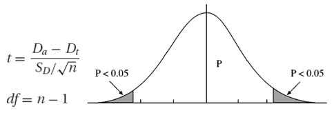
where n is the number of informative sites, df is the degree of freedom, t is the test statistical value, Da is the average site-to-site difference between the two trees, SD is the standard deviation, andDt is the total difference of branch lengths of the two trees.
Shimodaira–Hasegawa Test
A frequently used statistical test for ML trees is the Shimodaira–Hasegawa (SH) test (likelihood ratio test). It tests the goodness of fit of two competing trees using the χ2 test. For this test, log likelihood scores of two competing trees have to be obtained first. The degree of freedom used for the analysis depends on the substitution model used. It relies on the following test formula:
![]()
where d is the log likelihood ratio score and lnLA and lnLB are likelihood scores for tree A and tree B, respectively. The statistical meaning of d can be obtained from calculating the probability value from a χ2 table.
Once the log ratio of the two scores is obtained, it is used to test against the χ2 distribution. The resulting probability value (P-value) determines whether the difference between the two trees is significant.
Phylogenetic packages
This is a FREE package of programs for inferring phylogenies and carrying out certain related tasks. At present it contains 31 programs, which carry out different algorithms on different kinds of data. It is available free, from its Web site, in C source code, or as executables for Windows, Mac OS X, and Mac OS 8 or 9. The C source code can easily be compiled on Unix or Linux systems. It includes programs to carry out parsimony, distance matrix methods, maximum likelihood, and other methods on a variety of types of data, including DNA and RNA sequences, protein sequences, restriction sites, 0/1 discrete characters data, gene frequencies, continuous characters and distance matrices.
PAML
PAML (Phylogenetic analysis by Maximum Likelihood) is a package of programs for phylogenetic analyses of DNA or protein sequences using maximum likelihood. It is maintained and distributed for academic use free of charge by Ziheng Yang. ANSI C source codes are distributed for UNIX/Linux/Mac OSX, and executables are provided for MS Windows. PAML is not good for tree making.
MEGA
MEGA (Molecular Evolutionary Genetic Analysis) is produced by Sudhir Kumar of the Center for Evolutionary Functional Genomics of the The Biodesign Institute at Arizona State University, Tempe, Arizona (s.kumar (at) asu.edu) together with Joel Dudley of the Stanford Center for Biomedical Informatics Research at Stanford University, Koichiro Tamura of Tokyo Metropolitan University and Masatoshi Nei, of Pennsylvania State University. It carries out parsimony, distance matrix and likelihood methods for molecular data (nucleic acid sequences and protein sequences). It can do boostrapping, consensus trees, and a variety of distance measures, with Neighbor-Joining, Minimum Evolution, UPGMA, and parsimony tree methods, as a well as a large variety of data editing tasks, sequence alignment using an implementation of ClustalW, tests of the molecular clock, and single-branch tests of significance of groups. MEGA4 is the current version.
MacClade
MacClade is a pioneering program for interactive analysis of evolution of a variety of character types, including discrete characters and molecular sequences. It works on Macintoshes with Mac OS X, up to and including now Leopard, Mac OS X version 10.6 (and also on Mac OS). MacClade enables you to use the mouse-window interface to specify and rearrange phylogenies by hand, and watch the number of character steps and the distribution of states of a given character on the tree change as you do so. It has many other features beyond this, including ability to edit data, print out phylogenies, and even simulate the evolution of data on a tree.
PAUP (Phylogenetic Analysis Using Parsimony)
David Swofford of the School of Computational Science and Information Technology, Florida State University, Tallahassee, Florida has written PAUP (which originally meant Phylogenetic Analysis Using Parsimony). PAUP version 4.0beta10 has been released as a provisional version by Sinauer Associates, of Sunderland, Massachusetts. It has Macintosh, PowerMac, Windows, and Unix/OpenVMS versions. PAUP* has many options and close compatibility with MacClade. It includes parsimony, distance matrix, invariants, and maximum likelihood methods and many indices and statistical tests.